import numpy as np
import pandas as pd

import matplotlib.pyplot as plt
import plotly.express as px
from plotly.subplots import make_subplots
import plotly.io as pio
pio.renderers.defaule = 'colab'

from itables import showIntroduction to Data Science
Importing Recoding and Visualizing Data.
Important Information
- Email: joanna_bieri@redlands.edu
- Office Hours: Duke 209 Click Here for Joanna’s Schedule
Announcements
In about TWO WEEKS - Data Ethics We will start looking for resources.
Day 9 Assignment - same drill.
- Make sure Pull any new content from the class repo - then Copy it over into your working diretory.
- Open the file Day3-HW.ipynb and start doing the problems.
- You can do these problems as you follow along with the lecture notes and video.
- Get as far as you can before class.
- Submit what you have so far Commit and Push to Git.
- Take the daily check in quiz on Canvas.
- Come to class with lots of questions!
Data Science Visualization - from start to finish
Today we will do a fill analysis where we will import data, do some data cleaning (recoding), and then walk through how to create a really beautiful visualization.
Survey of religious traditions and income.
Source: pewforum.org/religious-landscape-study/income-distribution, Retrieved 14 April, 2020
This data is saved in a .xlsx file that is in the data folder that you downloaded.
This lab follows the Data Science in a Box lectures “Unit 2 - Deck 13: Recoding data” by Mine Çetinkaya-Rundel. It has been updated for our class and translated to Python by Joanna Bieri.
To use pd.read_excel() we need to download the openpyxl package:
#!conda install -y openpyxlfile_name = 'data/relig-income.xlsx'
DF = pd.read_excel(file_name)DF| Religious tradition | Less than $30,000 | $30,000-$49,999 | $50,000-$99,999 | $100,000 or more | Sample Size | |
|---|---|---|---|---|---|---|
| 0 | Buddhist | 0.36 | 0.18 | 0.32 | 0.13 | 233 |
| 1 | Catholic | 0.36 | 0.19 | 0.26 | 0.19 | 6137 |
| 2 | Evangelical Protestant | 0.35 | 0.22 | 0.28 | 0.14 | 7462 |
| 3 | Hindu | 0.17 | 0.13 | 0.34 | 0.36 | 172 |
| 4 | Historically Black Protestant | 0.53 | 0.22 | 0.17 | 0.08 | 1704 |
| 5 | Jehovah's Witness | 0.48 | 0.25 | 0.22 | 0.04 | 208 |
| 6 | Jewish | 0.16 | 0.15 | 0.24 | 0.44 | 708 |
| 7 | Mainline Protestant | 0.29 | 0.20 | 0.28 | 0.23 | 5208 |
| 8 | Mormon | 0.27 | 0.20 | 0.33 | 0.20 | 594 |
| 9 | Muslim | 0.34 | 0.17 | 0.29 | 0.20 | 205 |
| 10 | Orthodox Christian | 0.18 | 0.17 | 0.36 | 0.29 | 155 |
| 11 | Unaffiliated (religious "nones") | 0.33 | 0.20 | 0.26 | 0.21 | 6790 |
Q Describe the data you see here. How many variables and observations. What are the data types? What are the units?
Renaming Columns
Sometimes it is nice to give your columns easier to use names. If your data is downloaded with hard to remember or hard to type names it is more likely that you will make errors using those names later. I usually try to remove spaces in names and reduce the length of the names. We can use the .rename() function to do this:
DF.rename( columns={ 'old name 1':'new name 1' , 'old name 2':'new name 2' , 'old name 3':'new name 3', ... }, inplace=True )Here we use curly brackets {} to surround the names. You list the old name first then a colon then the new name. The flag inplace=True tells Python the change the data frame directly, not just in the print out. You can rename as many or as few columns as you want.
NOTE - This is also how you could rename your variables in your plots… just rename the columns.
DF.rename(columns={ 'Religious tradition':'religion' ,'Sample Size' : 'n' },inplace=True)
DF| religion | Less than $30,000 | $30,000-$49,999 | $50,000-$99,999 | $100,000 or more | n | |
|---|---|---|---|---|---|---|
| 0 | Buddhist | 0.36 | 0.18 | 0.32 | 0.13 | 233 |
| 1 | Catholic | 0.36 | 0.19 | 0.26 | 0.19 | 6137 |
| 2 | Evangelical Protestant | 0.35 | 0.22 | 0.28 | 0.14 | 7462 |
| 3 | Hindu | 0.17 | 0.13 | 0.34 | 0.36 | 172 |
| 4 | Historically Black Protestant | 0.53 | 0.22 | 0.17 | 0.08 | 1704 |
| 5 | Jehovah's Witness | 0.48 | 0.25 | 0.22 | 0.04 | 208 |
| 6 | Jewish | 0.16 | 0.15 | 0.24 | 0.44 | 708 |
| 7 | Mainline Protestant | 0.29 | 0.20 | 0.28 | 0.23 | 5208 |
| 8 | Mormon | 0.27 | 0.20 | 0.33 | 0.20 | 594 |
| 9 | Muslim | 0.34 | 0.17 | 0.29 | 0.20 | 205 |
| 10 | Orthodox Christian | 0.18 | 0.17 | 0.36 | 0.29 | 155 |
| 11 | Unaffiliated (religious "nones") | 0.33 | 0.20 | 0.26 | 0.21 | 6790 |
Pivots and Melts - Rearranging Data
Often the data we are given is in an order that is hard to use. To rearrange the data in our data frame we have two options
- The .pivot() reshapes your data so that one of the columns can become the row labels. To use the pivot method in Pandas, you need to specify three parameters:
- index: Which column should be used to identify and order your rows vertically
- columns: Which column should be used to create the new columns in our reshaped DataFrame.
- values: Which column(s) should be used to fill the values in the cells of our DataFrame.
- The pd.melt() can take column labels and melt them into your table values. To use the pd.melt() method in Pandas you need to specify three parameters:
- The DataFrame that you are melting
- id_vars the list of columns that should remain in your new data frame - used to index the unique rows.
- var_name the name of the new column that will hold the names of the new rows.
- value_name the name of the new column that will hold the values of the new rows
Pivot Example
Here is some example data of grades for three students over two exams. Let say the teacher keeps the data in a spreadsheet with three columns: First columns is the name, the second is the exam number, and the third is the grade on the exam. Here is an example of that data:
df = pd.DataFrame({'name': ['Alice', 'Bob', 'Eve', 'Eve', 'Alice', 'Bob'],
                   'exam': ['one', 'one', 'one', 'two', 'two','two'],
                   'grade': [92, 95, 70, 86, 90, 80]})

df| name | exam | grade | |
|---|---|---|---|
| 0 | Alice | one | 92 |
| 1 | Bob | one | 95 |
| 2 | Eve | one | 70 |
| 3 | Eve | two | 86 |
| 4 | Alice | two | 90 |
| 5 | Bob | two | 80 |
Now this is an okay to keep the data, but maybe we want to get more information about how each student is doing in the class and print a table of this data. To do this we need rearrange the data so that we get columns with the student names, rows for each exam and then inside the data frame the exam score. This is Pivoting.
Here is the plan:
- use index=‘name’ so that the names become the row labels (left hand side)
- use columns=‘exam’ so that the exams will become the column labels (top)
- use values=‘grade’ so that the grade will become the information in then table (inside)
- then add the average column
df_new = df.pivot(index='name', columns='exam', values='grade')
df_new| exam | one | two |
|---|---|---|
| name | ||
| Alice | 92 | 90 |
| Bob | 95 | 80 |
| Eve | 70 | 86 |
df_new['average']=(df_new['one']+df_new['two'])/2
df_new| exam | one | two | average |
|---|---|---|---|
| name | |||
| Alice | 92 | 90 | 91.0 |
| Bob | 95 | 80 | 87.5 |
| Eve | 70 | 86 | 78.0 |
Melt example
Here we have some example data where we have student grades across years and subjects. But maybe we really want to do an analysis of the overall scores in the program.
data = {'Name': ['Alice', 'Bob', 'Eve'],
        'Math_2022': [85, 90, 78],
        'Math_2023': [92, 88, 95],
        'Science_2022': [70, 82, 75],
        'Science_2023': [75, 85, 80]}

df = pd.DataFrame(data)
df| Name | Math_2022 | Math_2023 | Science_2022 | Science_2023 | |
|---|---|---|---|---|---|
| 0 | Alice | 85 | 92 | 70 | 75 |
| 1 | Bob | 90 | 88 | 82 | 85 |
| 2 | Eve | 78 | 95 | 75 | 80 |
So what we really want is all of the scores in a single column! Here is the plan:
- send the data frame df into pd.melt()
- use id_vars = [‘name’] so we still have a column with student names in it
- use var_name = ‘Subject_Year’ so the column that contains the subject and year information (all the other columns) will be labeled correctly.
- use value_name=‘Score’ so that we can take all the values (scores) and put them in one column named ‘Score’
df_new = pd.melt(df, id_vars=['Name'], var_name='Subject_Year', value_name='Score')
df_new| Name | Subject_Year | Score | |
|---|---|---|---|
| 0 | Alice | Math_2022 | 85 |
| 1 | Bob | Math_2022 | 90 |
| 2 | Eve | Math_2022 | 78 |
| 3 | Alice | Math_2023 | 92 |
| 4 | Bob | Math_2023 | 88 |
| 5 | Eve | Math_2023 | 95 |
| 6 | Alice | Science_2022 | 70 |
| 7 | Bob | Science_2022 | 82 |
| 8 | Eve | Science_2022 | 75 |
| 9 | Alice | Science_2023 | 75 |
| 10 | Bob | Science_2023 | 85 |
| 11 | Eve | Science_2023 | 80 |
You can see in both cases that by rearranging the data we made it visually more useful! How you arrange your data depends on the type of analysis you are trying to do.
Rearrange our Religions data
What we want for our data is all of the proportions (the values in the income columns) to be in a single row. We will use pd.melt() to do this!
NOTE: It takes some practice to get good at knowing just what will come out of a pivot() or melt(). Start by playing around with the command in this lecture. Change things and see what happens.
Look at the original data frame
DF| religion | Less than $30,000 | $30,000-$49,999 | $50,000-$99,999 | $100,000 or more | n | |
|---|---|---|---|---|---|---|
| 0 | Buddhist | 0.36 | 0.18 | 0.32 | 0.13 | 233 |
| 1 | Catholic | 0.36 | 0.19 | 0.26 | 0.19 | 6137 |
| 2 | Evangelical Protestant | 0.35 | 0.22 | 0.28 | 0.14 | 7462 |
| 3 | Hindu | 0.17 | 0.13 | 0.34 | 0.36 | 172 |
| 4 | Historically Black Protestant | 0.53 | 0.22 | 0.17 | 0.08 | 1704 |
| 5 | Jehovah's Witness | 0.48 | 0.25 | 0.22 | 0.04 | 208 |
| 6 | Jewish | 0.16 | 0.15 | 0.24 | 0.44 | 708 |
| 7 | Mainline Protestant | 0.29 | 0.20 | 0.28 | 0.23 | 5208 |
| 8 | Mormon | 0.27 | 0.20 | 0.33 | 0.20 | 594 |
| 9 | Muslim | 0.34 | 0.17 | 0.29 | 0.20 | 205 |
| 10 | Orthodox Christian | 0.18 | 0.17 | 0.36 | 0.29 | 155 |
| 11 | Unaffiliated (religious "nones") | 0.33 | 0.20 | 0.26 | 0.21 | 6790 |
Melt the data into a longer data frame.
In our final DataFrame we want to keep columns with information about ‘religion’ and ‘n’. We want to create TWO new columns, one that has the income levels (taken from the column names) and one that has the proportions (taken from the data table values). Here is the information we are sending in.
- DF
- id_vars=[‘religion’,‘n’] - keep these columns
- var_name=‘income’ - make a column using all the other variables (column names) - name that column income
- value_name=‘proportion’ - make a column using all the other values (stuff inside the table) - name that column proportion
Note - I am also going to sort it by religion to make it nice to read.
DF_new = pd.melt(DF, id_vars=['religion','n'], var_name='income', value_name='proportion').sort_values('religion')
DF_new| religion | n | income | proportion | |
|---|---|---|---|---|
| 0 | Buddhist | 233 | Less than $30,000 | 0.36 |
| 24 | Buddhist | 233 | $50,000-$99,999 | 0.32 |
| 36 | Buddhist | 233 | $100,000 or more | 0.13 |
| 12 | Buddhist | 233 | $30,000-$49,999 | 0.18 |
| 1 | Catholic | 6137 | Less than $30,000 | 0.36 |
| 25 | Catholic | 6137 | $50,000-$99,999 | 0.26 |
| 13 | Catholic | 6137 | $30,000-$49,999 | 0.19 |
| 37 | Catholic | 6137 | $100,000 or more | 0.19 |
| 26 | Evangelical Protestant | 7462 | $50,000-$99,999 | 0.28 |
| 38 | Evangelical Protestant | 7462 | $100,000 or more | 0.14 |
| 14 | Evangelical Protestant | 7462 | $30,000-$49,999 | 0.22 |
| 2 | Evangelical Protestant | 7462 | Less than $30,000 | 0.35 |
| 3 | Hindu | 172 | Less than $30,000 | 0.17 |
| 27 | Hindu | 172 | $50,000-$99,999 | 0.34 |
| 15 | Hindu | 172 | $30,000-$49,999 | 0.13 |
| 39 | Hindu | 172 | $100,000 or more | 0.36 |
| 40 | Historically Black Protestant | 1704 | $100,000 or more | 0.08 |
| 4 | Historically Black Protestant | 1704 | Less than $30,000 | 0.53 |
| 28 | Historically Black Protestant | 1704 | $50,000-$99,999 | 0.17 |
| 16 | Historically Black Protestant | 1704 | $30,000-$49,999 | 0.22 |
| 17 | Jehovah's Witness | 208 | $30,000-$49,999 | 0.25 |
| 29 | Jehovah's Witness | 208 | $50,000-$99,999 | 0.22 |
| 41 | Jehovah's Witness | 208 | $100,000 or more | 0.04 |
| 5 | Jehovah's Witness | 208 | Less than $30,000 | 0.48 |
| 42 | Jewish | 708 | $100,000 or more | 0.44 |
| 30 | Jewish | 708 | $50,000-$99,999 | 0.24 |
| 6 | Jewish | 708 | Less than $30,000 | 0.16 |
| 18 | Jewish | 708 | $30,000-$49,999 | 0.15 |
| 31 | Mainline Protestant | 5208 | $50,000-$99,999 | 0.28 |
| 43 | Mainline Protestant | 5208 | $100,000 or more | 0.23 |
| 19 | Mainline Protestant | 5208 | $30,000-$49,999 | 0.20 |
| 7 | Mainline Protestant | 5208 | Less than $30,000 | 0.29 |
| 20 | Mormon | 594 | $30,000-$49,999 | 0.20 |
| 32 | Mormon | 594 | $50,000-$99,999 | 0.33 |
| 44 | Mormon | 594 | $100,000 or more | 0.20 |
| 8 | Mormon | 594 | Less than $30,000 | 0.27 |
| 33 | Muslim | 205 | $50,000-$99,999 | 0.29 |
| 45 | Muslim | 205 | $100,000 or more | 0.20 |
| 9 | Muslim | 205 | Less than $30,000 | 0.34 |
| 21 | Muslim | 205 | $30,000-$49,999 | 0.17 |
| 22 | Orthodox Christian | 155 | $30,000-$49,999 | 0.17 |
| 34 | Orthodox Christian | 155 | $50,000-$99,999 | 0.36 |
| 10 | Orthodox Christian | 155 | Less than $30,000 | 0.18 |
| 46 | Orthodox Christian | 155 | $100,000 or more | 0.29 |
| 23 | Unaffiliated (religious "nones") | 6790 | $30,000-$49,999 | 0.20 |
| 11 | Unaffiliated (religious "nones") | 6790 | Less than $30,000 | 0.33 |
| 35 | Unaffiliated (religious "nones") | 6790 | $50,000-$99,999 | 0.26 |
| 47 | Unaffiliated (religious "nones") | 6790 | $100,000 or more | 0.21 |
Lets add an extra column
We can calculate the frequency of observations by multiplying the proportion column by the n (the sample size).
NOTE: Technically because of rounding we may have some data that does not quite add up. We will accept this possible error for now.
DF_new['frequency']=np.round(DF_new['proportion']*DF_new['n'])
DF_new| religion | n | income | proportion | frequency | |
|---|---|---|---|---|---|
| 0 | Buddhist | 233 | Less than $30,000 | 0.36 | 84.0 |
| 24 | Buddhist | 233 | $50,000-$99,999 | 0.32 | 75.0 |
| 36 | Buddhist | 233 | $100,000 or more | 0.13 | 30.0 |
| 12 | Buddhist | 233 | $30,000-$49,999 | 0.18 | 42.0 |
| 1 | Catholic | 6137 | Less than $30,000 | 0.36 | 2209.0 |
| 25 | Catholic | 6137 | $50,000-$99,999 | 0.26 | 1596.0 |
| 13 | Catholic | 6137 | $30,000-$49,999 | 0.19 | 1166.0 |
| 37 | Catholic | 6137 | $100,000 or more | 0.19 | 1166.0 |
| 26 | Evangelical Protestant | 7462 | $50,000-$99,999 | 0.28 | 2089.0 |
| 38 | Evangelical Protestant | 7462 | $100,000 or more | 0.14 | 1045.0 |
| 14 | Evangelical Protestant | 7462 | $30,000-$49,999 | 0.22 | 1642.0 |
| 2 | Evangelical Protestant | 7462 | Less than $30,000 | 0.35 | 2612.0 |
| 3 | Hindu | 172 | Less than $30,000 | 0.17 | 29.0 |
| 27 | Hindu | 172 | $50,000-$99,999 | 0.34 | 58.0 |
| 15 | Hindu | 172 | $30,000-$49,999 | 0.13 | 22.0 |
| 39 | Hindu | 172 | $100,000 or more | 0.36 | 62.0 |
| 40 | Historically Black Protestant | 1704 | $100,000 or more | 0.08 | 136.0 |
| 4 | Historically Black Protestant | 1704 | Less than $30,000 | 0.53 | 903.0 |
| 28 | Historically Black Protestant | 1704 | $50,000-$99,999 | 0.17 | 290.0 |
| 16 | Historically Black Protestant | 1704 | $30,000-$49,999 | 0.22 | 375.0 |
| 17 | Jehovah's Witness | 208 | $30,000-$49,999 | 0.25 | 52.0 |
| 29 | Jehovah's Witness | 208 | $50,000-$99,999 | 0.22 | 46.0 |
| 41 | Jehovah's Witness | 208 | $100,000 or more | 0.04 | 8.0 |
| 5 | Jehovah's Witness | 208 | Less than $30,000 | 0.48 | 100.0 |
| 42 | Jewish | 708 | $100,000 or more | 0.44 | 312.0 |
| 30 | Jewish | 708 | $50,000-$99,999 | 0.24 | 170.0 |
| 6 | Jewish | 708 | Less than $30,000 | 0.16 | 113.0 |
| 18 | Jewish | 708 | $30,000-$49,999 | 0.15 | 106.0 |
| 31 | Mainline Protestant | 5208 | $50,000-$99,999 | 0.28 | 1458.0 |
| 43 | Mainline Protestant | 5208 | $100,000 or more | 0.23 | 1198.0 |
| 19 | Mainline Protestant | 5208 | $30,000-$49,999 | 0.20 | 1042.0 |
| 7 | Mainline Protestant | 5208 | Less than $30,000 | 0.29 | 1510.0 |
| 20 | Mormon | 594 | $30,000-$49,999 | 0.20 | 119.0 |
| 32 | Mormon | 594 | $50,000-$99,999 | 0.33 | 196.0 |
| 44 | Mormon | 594 | $100,000 or more | 0.20 | 119.0 |
| 8 | Mormon | 594 | Less than $30,000 | 0.27 | 160.0 |
| 33 | Muslim | 205 | $50,000-$99,999 | 0.29 | 59.0 |
| 45 | Muslim | 205 | $100,000 or more | 0.20 | 41.0 |
| 9 | Muslim | 205 | Less than $30,000 | 0.34 | 70.0 |
| 21 | Muslim | 205 | $30,000-$49,999 | 0.17 | 35.0 |
| 22 | Orthodox Christian | 155 | $30,000-$49,999 | 0.17 | 26.0 |
| 34 | Orthodox Christian | 155 | $50,000-$99,999 | 0.36 | 56.0 |
| 10 | Orthodox Christian | 155 | Less than $30,000 | 0.18 | 28.0 |
| 46 | Orthodox Christian | 155 | $100,000 or more | 0.29 | 45.0 |
| 23 | Unaffiliated (religious "nones") | 6790 | $30,000-$49,999 | 0.20 | 1358.0 |
| 11 | Unaffiliated (religious "nones") | 6790 | Less than $30,000 | 0.33 | 2241.0 |
| 35 | Unaffiliated (religious "nones") | 6790 | $50,000-$99,999 | 0.26 | 1765.0 |
| 47 | Unaffiliated (religious "nones") | 6790 | $100,000 or more | 0.21 | 1426.0 |
Get rid of those dolar signs to make the text consistent
DF_new['income']=DF_new['income'].apply(lambda x: str(x).replace('$',''))
DF_new| religion | n | income | proportion | frequency | |
|---|---|---|---|---|---|
| 0 | Buddhist | 233 | Less than 30,000 | 0.36 | 84.0 |
| 24 | Buddhist | 233 | 50,000-99,999 | 0.32 | 75.0 |
| 36 | Buddhist | 233 | 100,000 or more | 0.13 | 30.0 |
| 12 | Buddhist | 233 | 30,000-49,999 | 0.18 | 42.0 |
| 1 | Catholic | 6137 | Less than 30,000 | 0.36 | 2209.0 |
| 25 | Catholic | 6137 | 50,000-99,999 | 0.26 | 1596.0 |
| 13 | Catholic | 6137 | 30,000-49,999 | 0.19 | 1166.0 |
| 37 | Catholic | 6137 | 100,000 or more | 0.19 | 1166.0 |
| 26 | Evangelical Protestant | 7462 | 50,000-99,999 | 0.28 | 2089.0 |
| 38 | Evangelical Protestant | 7462 | 100,000 or more | 0.14 | 1045.0 |
| 14 | Evangelical Protestant | 7462 | 30,000-49,999 | 0.22 | 1642.0 |
| 2 | Evangelical Protestant | 7462 | Less than 30,000 | 0.35 | 2612.0 |
| 3 | Hindu | 172 | Less than 30,000 | 0.17 | 29.0 |
| 27 | Hindu | 172 | 50,000-99,999 | 0.34 | 58.0 |
| 15 | Hindu | 172 | 30,000-49,999 | 0.13 | 22.0 |
| 39 | Hindu | 172 | 100,000 or more | 0.36 | 62.0 |
| 40 | Historically Black Protestant | 1704 | 100,000 or more | 0.08 | 136.0 |
| 4 | Historically Black Protestant | 1704 | Less than 30,000 | 0.53 | 903.0 |
| 28 | Historically Black Protestant | 1704 | 50,000-99,999 | 0.17 | 290.0 |
| 16 | Historically Black Protestant | 1704 | 30,000-49,999 | 0.22 | 375.0 |
| 17 | Jehovah's Witness | 208 | 30,000-49,999 | 0.25 | 52.0 |
| 29 | Jehovah's Witness | 208 | 50,000-99,999 | 0.22 | 46.0 |
| 41 | Jehovah's Witness | 208 | 100,000 or more | 0.04 | 8.0 |
| 5 | Jehovah's Witness | 208 | Less than 30,000 | 0.48 | 100.0 |
| 42 | Jewish | 708 | 100,000 or more | 0.44 | 312.0 |
| 30 | Jewish | 708 | 50,000-99,999 | 0.24 | 170.0 |
| 6 | Jewish | 708 | Less than 30,000 | 0.16 | 113.0 |
| 18 | Jewish | 708 | 30,000-49,999 | 0.15 | 106.0 |
| 31 | Mainline Protestant | 5208 | 50,000-99,999 | 0.28 | 1458.0 |
| 43 | Mainline Protestant | 5208 | 100,000 or more | 0.23 | 1198.0 |
| 19 | Mainline Protestant | 5208 | 30,000-49,999 | 0.20 | 1042.0 |
| 7 | Mainline Protestant | 5208 | Less than 30,000 | 0.29 | 1510.0 |
| 20 | Mormon | 594 | 30,000-49,999 | 0.20 | 119.0 |
| 32 | Mormon | 594 | 50,000-99,999 | 0.33 | 196.0 |
| 44 | Mormon | 594 | 100,000 or more | 0.20 | 119.0 |
| 8 | Mormon | 594 | Less than 30,000 | 0.27 | 160.0 |
| 33 | Muslim | 205 | 50,000-99,999 | 0.29 | 59.0 |
| 45 | Muslim | 205 | 100,000 or more | 0.20 | 41.0 |
| 9 | Muslim | 205 | Less than 30,000 | 0.34 | 70.0 |
| 21 | Muslim | 205 | 30,000-49,999 | 0.17 | 35.0 |
| 22 | Orthodox Christian | 155 | 30,000-49,999 | 0.17 | 26.0 |
| 34 | Orthodox Christian | 155 | 50,000-99,999 | 0.36 | 56.0 |
| 10 | Orthodox Christian | 155 | Less than 30,000 | 0.18 | 28.0 |
| 46 | Orthodox Christian | 155 | 100,000 or more | 0.29 | 45.0 |
| 23 | Unaffiliated (religious "nones") | 6790 | 30,000-49,999 | 0.20 | 1358.0 |
| 11 | Unaffiliated (religious "nones") | 6790 | Less than 30,000 | 0.33 | 2241.0 |
| 35 | Unaffiliated (religious "nones") | 6790 | 50,000-99,999 | 0.26 | 1765.0 |
| 47 | Unaffiliated (religious "nones") | 6790 | 100,000 or more | 0.21 | 1426.0 |
Reset the index.
Resetting the index makes the numbers on the left hand side in order from 0 to 47, instead of them being based on the original data frame that was not sorted alphabetically.
DF_new.reset_index(inplace=True)
DF_new| index | religion | n | income | proportion | frequency | |
|---|---|---|---|---|---|---|
| 0 | 0 | Buddhist | 233 | Less than 30,000 | 0.36 | 84.0 |
| 1 | 24 | Buddhist | 233 | 50,000-99,999 | 0.32 | 75.0 |
| 2 | 36 | Buddhist | 233 | 100,000 or more | 0.13 | 30.0 |
| 3 | 12 | Buddhist | 233 | 30,000-49,999 | 0.18 | 42.0 |
| 4 | 1 | Catholic | 6137 | Less than 30,000 | 0.36 | 2209.0 |
| 5 | 25 | Catholic | 6137 | 50,000-99,999 | 0.26 | 1596.0 |
| 6 | 13 | Catholic | 6137 | 30,000-49,999 | 0.19 | 1166.0 |
| 7 | 37 | Catholic | 6137 | 100,000 or more | 0.19 | 1166.0 |
| 8 | 26 | Evangelical Protestant | 7462 | 50,000-99,999 | 0.28 | 2089.0 |
| 9 | 38 | Evangelical Protestant | 7462 | 100,000 or more | 0.14 | 1045.0 |
| 10 | 14 | Evangelical Protestant | 7462 | 30,000-49,999 | 0.22 | 1642.0 |
| 11 | 2 | Evangelical Protestant | 7462 | Less than 30,000 | 0.35 | 2612.0 |
| 12 | 3 | Hindu | 172 | Less than 30,000 | 0.17 | 29.0 |
| 13 | 27 | Hindu | 172 | 50,000-99,999 | 0.34 | 58.0 |
| 14 | 15 | Hindu | 172 | 30,000-49,999 | 0.13 | 22.0 |
| 15 | 39 | Hindu | 172 | 100,000 or more | 0.36 | 62.0 |
| 16 | 40 | Historically Black Protestant | 1704 | 100,000 or more | 0.08 | 136.0 |
| 17 | 4 | Historically Black Protestant | 1704 | Less than 30,000 | 0.53 | 903.0 |
| 18 | 28 | Historically Black Protestant | 1704 | 50,000-99,999 | 0.17 | 290.0 |
| 19 | 16 | Historically Black Protestant | 1704 | 30,000-49,999 | 0.22 | 375.0 |
| 20 | 17 | Jehovah's Witness | 208 | 30,000-49,999 | 0.25 | 52.0 |
| 21 | 29 | Jehovah's Witness | 208 | 50,000-99,999 | 0.22 | 46.0 |
| 22 | 41 | Jehovah's Witness | 208 | 100,000 or more | 0.04 | 8.0 |
| 23 | 5 | Jehovah's Witness | 208 | Less than 30,000 | 0.48 | 100.0 |
| 24 | 42 | Jewish | 708 | 100,000 or more | 0.44 | 312.0 |
| 25 | 30 | Jewish | 708 | 50,000-99,999 | 0.24 | 170.0 |
| 26 | 6 | Jewish | 708 | Less than 30,000 | 0.16 | 113.0 |
| 27 | 18 | Jewish | 708 | 30,000-49,999 | 0.15 | 106.0 |
| 28 | 31 | Mainline Protestant | 5208 | 50,000-99,999 | 0.28 | 1458.0 |
| 29 | 43 | Mainline Protestant | 5208 | 100,000 or more | 0.23 | 1198.0 |
| 30 | 19 | Mainline Protestant | 5208 | 30,000-49,999 | 0.20 | 1042.0 |
| 31 | 7 | Mainline Protestant | 5208 | Less than 30,000 | 0.29 | 1510.0 |
| 32 | 20 | Mormon | 594 | 30,000-49,999 | 0.20 | 119.0 |
| 33 | 32 | Mormon | 594 | 50,000-99,999 | 0.33 | 196.0 |
| 34 | 44 | Mormon | 594 | 100,000 or more | 0.20 | 119.0 |
| 35 | 8 | Mormon | 594 | Less than 30,000 | 0.27 | 160.0 |
| 36 | 33 | Muslim | 205 | 50,000-99,999 | 0.29 | 59.0 |
| 37 | 45 | Muslim | 205 | 100,000 or more | 0.20 | 41.0 |
| 38 | 9 | Muslim | 205 | Less than 30,000 | 0.34 | 70.0 |
| 39 | 21 | Muslim | 205 | 30,000-49,999 | 0.17 | 35.0 |
| 40 | 22 | Orthodox Christian | 155 | 30,000-49,999 | 0.17 | 26.0 |
| 41 | 34 | Orthodox Christian | 155 | 50,000-99,999 | 0.36 | 56.0 |
| 42 | 10 | Orthodox Christian | 155 | Less than 30,000 | 0.18 | 28.0 |
| 43 | 46 | Orthodox Christian | 155 | 100,000 or more | 0.29 | 45.0 |
| 44 | 23 | Unaffiliated (religious "nones") | 6790 | 30,000-49,999 | 0.20 | 1358.0 |
| 45 | 11 | Unaffiliated (religious "nones") | 6790 | Less than 30,000 | 0.33 | 2241.0 |
| 46 | 35 | Unaffiliated (religious "nones") | 6790 | 50,000-99,999 | 0.26 | 1765.0 |
| 47 | 47 | Unaffiliated (religious "nones") | 6790 | 100,000 or more | 0.21 | 1426.0 |
Make a Bar Plot
Here is another example of building up a plot. Starting simple and slowly adding features until we have a really nice looking plot!
Put the religions on the y-axis
We will plot the data with the categorical data on the y-axis since the names are a little longer. This will make the names easier to read!
fig = px.bar(DF_new,y='religion',x='frequency',color_discrete_sequence=['gray'])

fig.update_layout(xaxis_title="Frequency",
                  yaxis_title="Religion",
                  autosize=False,
                  width=800,
                  height=500)

fig.show()
Unable to display output for mime type(s): application/vnd.plotly.v1+jsonRename some of the categories
Some of the religion names are really long, making them a bit harder to read. We can do this using the .replace() method.
DF.replace('old word','new word')name_to_change = 'Unaffiliated (religious "nones")'
new_name = 'Unaffiliated'
DF_new['religion']=DF_new['religion'].replace(name_to_change,new_name)
name_to_change = 'Historically Black Protestant'
new_name = 'Hist. Black Protestant'
DF_new['religion']=DF_new['religion'].replace(name_to_change,new_name)
name_to_change = 'Evangelical Protestant'
new_name = 'Ev. Protestant'
DF_new['religion']=DF_new['religion'].replace(name_to_change,new_name)
DF_new| index | religion | n | income | proportion | frequency | |
|---|---|---|---|---|---|---|
| 0 | 0 | Buddhist | 233 | Less than 30,000 | 0.36 | 84.0 |
| 1 | 24 | Buddhist | 233 | 50,000-99,999 | 0.32 | 75.0 |
| 2 | 36 | Buddhist | 233 | 100,000 or more | 0.13 | 30.0 |
| 3 | 12 | Buddhist | 233 | 30,000-49,999 | 0.18 | 42.0 |
| 4 | 1 | Catholic | 6137 | Less than 30,000 | 0.36 | 2209.0 |
| 5 | 25 | Catholic | 6137 | 50,000-99,999 | 0.26 | 1596.0 |
| 6 | 13 | Catholic | 6137 | 30,000-49,999 | 0.19 | 1166.0 |
| 7 | 37 | Catholic | 6137 | 100,000 or more | 0.19 | 1166.0 |
| 8 | 26 | Ev. Protestant | 7462 | 50,000-99,999 | 0.28 | 2089.0 |
| 9 | 38 | Ev. Protestant | 7462 | 100,000 or more | 0.14 | 1045.0 |
| 10 | 14 | Ev. Protestant | 7462 | 30,000-49,999 | 0.22 | 1642.0 |
| 11 | 2 | Ev. Protestant | 7462 | Less than 30,000 | 0.35 | 2612.0 |
| 12 | 3 | Hindu | 172 | Less than 30,000 | 0.17 | 29.0 |
| 13 | 27 | Hindu | 172 | 50,000-99,999 | 0.34 | 58.0 |
| 14 | 15 | Hindu | 172 | 30,000-49,999 | 0.13 | 22.0 |
| 15 | 39 | Hindu | 172 | 100,000 or more | 0.36 | 62.0 |
| 16 | 40 | Hist. Black Protestant | 1704 | 100,000 or more | 0.08 | 136.0 |
| 17 | 4 | Hist. Black Protestant | 1704 | Less than 30,000 | 0.53 | 903.0 |
| 18 | 28 | Hist. Black Protestant | 1704 | 50,000-99,999 | 0.17 | 290.0 |
| 19 | 16 | Hist. Black Protestant | 1704 | 30,000-49,999 | 0.22 | 375.0 |
| 20 | 17 | Jehovah's Witness | 208 | 30,000-49,999 | 0.25 | 52.0 |
| 21 | 29 | Jehovah's Witness | 208 | 50,000-99,999 | 0.22 | 46.0 |
| 22 | 41 | Jehovah's Witness | 208 | 100,000 or more | 0.04 | 8.0 |
| 23 | 5 | Jehovah's Witness | 208 | Less than 30,000 | 0.48 | 100.0 |
| 24 | 42 | Jewish | 708 | 100,000 or more | 0.44 | 312.0 |
| 25 | 30 | Jewish | 708 | 50,000-99,999 | 0.24 | 170.0 |
| 26 | 6 | Jewish | 708 | Less than 30,000 | 0.16 | 113.0 |
| 27 | 18 | Jewish | 708 | 30,000-49,999 | 0.15 | 106.0 |
| 28 | 31 | Mainline Protestant | 5208 | 50,000-99,999 | 0.28 | 1458.0 |
| 29 | 43 | Mainline Protestant | 5208 | 100,000 or more | 0.23 | 1198.0 |
| 30 | 19 | Mainline Protestant | 5208 | 30,000-49,999 | 0.20 | 1042.0 |
| 31 | 7 | Mainline Protestant | 5208 | Less than 30,000 | 0.29 | 1510.0 |
| 32 | 20 | Mormon | 594 | 30,000-49,999 | 0.20 | 119.0 |
| 33 | 32 | Mormon | 594 | 50,000-99,999 | 0.33 | 196.0 |
| 34 | 44 | Mormon | 594 | 100,000 or more | 0.20 | 119.0 |
| 35 | 8 | Mormon | 594 | Less than 30,000 | 0.27 | 160.0 |
| 36 | 33 | Muslim | 205 | 50,000-99,999 | 0.29 | 59.0 |
| 37 | 45 | Muslim | 205 | 100,000 or more | 0.20 | 41.0 |
| 38 | 9 | Muslim | 205 | Less than 30,000 | 0.34 | 70.0 |
| 39 | 21 | Muslim | 205 | 30,000-49,999 | 0.17 | 35.0 |
| 40 | 22 | Orthodox Christian | 155 | 30,000-49,999 | 0.17 | 26.0 |
| 41 | 34 | Orthodox Christian | 155 | 50,000-99,999 | 0.36 | 56.0 |
| 42 | 10 | Orthodox Christian | 155 | Less than 30,000 | 0.18 | 28.0 |
| 43 | 46 | Orthodox Christian | 155 | 100,000 or more | 0.29 | 45.0 |
| 44 | 23 | Unaffiliated | 6790 | 30,000-49,999 | 0.20 | 1358.0 |
| 45 | 11 | Unaffiliated | 6790 | Less than 30,000 | 0.33 | 2241.0 |
| 46 | 35 | Unaffiliated | 6790 | 50,000-99,999 | 0.26 | 1765.0 |
| 47 | 47 | Unaffiliated | 6790 | 100,000 or more | 0.21 | 1426.0 |
fig = px.bar(DF_new,y='religion',x='frequency',color_discrete_sequence=['gray'])

fig.update_layout(xaxis_title="Frequency",
                  yaxis_title="Religion",
                  autosize=False,
                  width=800,
                  height=500)

fig.show()
Unable to display output for mime type(s): application/vnd.plotly.v1+jsonReverse the order of the categories
Here we see that to read this alphabetically we have to read up from the bottom. Mathematically it makes sense to count along the y-axis starting from zero, but with words it seems a little bit strange. We can do this in the figure layout. We just add:
yaxis={'categoryorder': 'category descending'}we can also change ‘category descending’ to ‘category ascending’ if we wanted to foce ascending. And we could change from yaxis to xaxis if we had categories along the x-axis.
fig = px.bar(DF_new,y='religion',x='frequency',color_discrete_sequence=['gray'])

fig.update_layout(yaxis={'categoryorder': 'category descending'},
                  xaxis_title="Frequency",
                  yaxis_title="Religion",
                  autosize=False,
                  width=800,
                  height=500)

fig.show()
Unable to display output for mime type(s): application/vnd.plotly.v1+jsonAdd the income information in color
fig = px.bar(DF_new,y='religion',x='frequency',color='income')

fig.update_layout(yaxis={'categoryorder': 'category descending'},
                  xaxis_title="Frequency",
                  yaxis_title="Religion",
                  autosize=False,
                  width=800,
                  height=500)

fig.show()
Unable to display output for mime type(s): application/vnd.plotly.v1+jsonLet’s fix those category orders
Here is how you can get a quick list of all the income brackets:
list(DF_new['income'].drop_duplicates())['Less than 30,000', '50,000-99,999', '100,000 or more', '30,000-49,999']Then we can fix the category order using the command
category_orders={'income' : ['Less than 30,000', '30,000-49,999', '50,000-99,999', '100,000 or more']}notice how I changed the order of the last bracket ‘30,000-49,999’ so that it appears second.
fig = px.bar(DF_new,
             y='religion',
             x='frequency',
             color='income',
             category_orders={'income' : ['Less than 30,000', '30,000-49,999', '50,000-99,999', '100,000 or more']})

fig.update_layout(yaxis={'categoryorder': 'category descending'},
                  xaxis_title="Frequency",
                  yaxis_title="Religion",
                  legend_title='Income',
                  autosize=False,
                  width=800,
                  height=500)

fig.show()
Unable to display output for mime type(s): application/vnd.plotly.v1+jsonConsider proportions instead of frequencies
fig = px.bar(DF_new,
             y='religion',
             x='proportion',
             color='income',
             category_orders={'income' : ['Less than 30,000', '30,000-49,999', '50,000-99,999', '100,000 or more']})

fig.update_layout(yaxis={'categoryorder': 'category descending'},
                  xaxis_title="Proportion",
                  yaxis_title="Religion",
                  legend_title='Income',
                  autosize=False,
                  width=800,
                  height=500)

fig.show()
Unable to display output for mime type(s): application/vnd.plotly.v1+jsonQ What different information do we get from the Frequency vs. the Proportion bar plots?
Try some new colors
We can add a built in color sequence using the command:
color_discrete_sequence=px.colors.qualitative.VividIn this example we picked the ‘Vivid’ color sequence. See below for more choices!
fig = px.bar(DF_new,
             y='religion',
             x='proportion',
             color='income',
             color_discrete_sequence=px.colors.qualitative.Vivid,
             category_orders={'income' : ['Less than 30,000', '30,000-49,999', '50,000-99,999', '100,000 or more']})

fig.update_layout(yaxis={'categoryorder': 'category descending'},
                  xaxis_title="Proportion",
                  yaxis_title="Religion",
                  legend_title='Income',
                  autosize=False,
                  width=800,
                  height=500)

fig.show()
Unable to display output for mime type(s): application/vnd.plotly.v1+jsonfig = px.colors.qualitative.swatches()
fig.show()Unable to display output for mime type(s): application/vnd.plotly.v1+jsonApply Templates to make the plot look even nicer
fig = px.bar(DF_new,
             y='religion',
             x='proportion',
             color='income',
             color_discrete_sequence=px.colors.qualitative.Vivid,
             category_orders={'income' : ['Less than 30,000', '30,000-49,999', '50,000-99,999', '100,000 or more']})

fig.update_layout(template="plotly_white",
                  yaxis={'categoryorder': 'category descending'},
                  xaxis_title="Proportion",
                  yaxis_title="Religion",
                  legend_title='Income',
                  autosize=False,
                  width=800,
                  height=500)

fig.show()
Unable to display output for mime type(s): application/vnd.plotly.v1+jsonHere is an example of our plots using a few different templates
for template in ["plotly", "plotly_white", "plotly_dark", "ggplot2", "seaborn", "simple_white"]:

    print(f'Template Name = {template}')

    fig = px.bar(DF_new,
                 y='religion',
                 x='proportion',
                 color='income',
                 color_discrete_sequence=px.colors.qualitative.Vivid,
                 category_orders={'income' : ['Less than 30,000', '30,000-49,999', '50,000-99,999', '100,000 or more']})

    fig.update_layout(template=template,
                      yaxis={'categoryorder': 'category descending'},
                      xaxis_title="Proportion",
                      yaxis_title="Religion",
                      legend_title='Income',
                      autosize=False,
                      width=800,
                      height=500)

    fig.show()
Template Name = plotly
Template Name = plotly_white
Template Name = plotly_dark
Template Name = ggplot2
Template Name = seaborn
Template Name = simple_whiteUnable to display output for mime type(s): application/vnd.plotly.v1+jsonUnable to display output for mime type(s): application/vnd.plotly.v1+jsonUnable to display output for mime type(s): application/vnd.plotly.v1+jsonUnable to display output for mime type(s): application/vnd.plotly.v1+jsonUnable to display output for mime type(s): application/vnd.plotly.v1+jsonUnable to display output for mime type(s): application/vnd.plotly.v1+jsonMoving the legend.
Plotly will let you place the legend exactly where you want it using the legend layout information:
- ‘orientation’:“h” - “h” means horizontal, “v” means vertical
- x and y anchor tells plotly where the (0,0) point is. So if we want to put our legend at the bottom right we would use:
- ‘yanchor’:“bottom”
- ‘xanchor’:“right”
- The we can move the legend around using x and y:
- ‘y’:1.05 - this would shift up above the plot
- ‘x’:0.95 - this would shift left almost to the left of the plot.
Move the legend from the side to the top
fig = px.bar(DF_new,
             y='religion',
             x='proportion',
             color='income',
             color_discrete_sequence=px.colors.qualitative.Vivid,
             category_orders={'income' : ['Less than 30,000', '30,000-49,999', '50,000-99,999', '100,000 or more']})

fig.update_layout(template="plotly_white",
                  yaxis={'categoryorder': 'category descending'},
                  xaxis_title="Proportion",
                  yaxis_title="Religion",
                  legend_title='Income',
                  legend={'orientation':"h",'yanchor':"bottom",'y':1.05, 'xanchor':"right",'x':0.95},
                  autosize=False,
                  width=800,
                  height=500)

fig.show()
Unable to display output for mime type(s): application/vnd.plotly.v1+jsonMove the legend from the side to the Bottom
fig = px.bar(DF_new,
             y='religion',
             x='proportion',
             color='income',
             color_discrete_sequence=px.colors.qualitative.Vivid,
             category_orders={'income' : ['Less than 30,000', '30,000-49,999', '50,000-99,999', '100,000 or more']})

fig.update_layout(template="plotly_white",
                  yaxis={'categoryorder': 'category descending'},
                  xaxis_title="Proportion",
                  yaxis_title="Religion",
                  legend_title='Income',
                  legend={'orientation':"h",'yanchor':"bottom",'y':-0.3, 'xanchor':"right",'x':0.95},
                  autosize=False,
                  width=800,
                  height=500)

fig.show()
Unable to display output for mime type(s): application/vnd.plotly.v1+jsonThere are SO MANY CUSTOMIZATION OPTIONS!
You are not expected to have all of these options memorized. You should just know that these things are possible and then look up examples for how to do fancier things. I always start simple and then add on from there.
Final Plot
fig = px.bar(DF_new,
             y='religion',
             x='proportion',
             color='income',
             color_discrete_sequence=px.colors.qualitative.Vivid,
             category_orders={'income' : ['Less than 30,000', '30,000-49,999', '50,000-99,999', '100,000 or more']})

fig.update_layout(template="plotly_white",
                  title='Income Distribution by religious group <br><sup>Data Source: Pew Research Center, Religious Lansdcape Study</sup>',
                  title_x=0.5,
                  yaxis={'categoryorder': 'category descending'},
                  xaxis_title="Proportion",
                  yaxis_title="",
                  legend_title='Income',
                  legend={'orientation':"h",'yanchor':"bottom",'y':-0.2, 'xanchor':"right",'x':1.05},
                  font={'family':"Courier New, monospace",'size':16,'color':"Darkblue"},
                  autosize=False,
                  width=1000,
                  height=800)

fig.show()
Unable to display output for mime type(s): application/vnd.plotly.v1+jsonExercise 1
Make your own version of the plot above. Here are some changes you should try:
Change the font family - some common fonts to try:
  ["Arial",
  "Balto",
  "Courier New",
  "Droid Sans",
  "Droid Serif",
  "Droid Sans Mono",
  "Gravitas One",
  "Old Standard TT",
  "Open Sans",
  "Overpass",
  "PT Sans Narrow",
  "Raleway",
  "Times New Roman"]
Move the legend to somewhere else.
Change the template and the color.
Advanced - look up how you can change the pattern_shape or pattern_shape_sequence.
Exercise 2
In this exercise we are going to import some very messy data and see how we can Recode, Tidy, and Pivot the data!
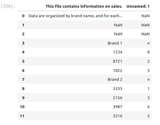
1. Import the data from the file: file_name = ‘data/sales.xlsx’
Look at the DataFrame, the data is not in a great format. Why is this data not tidy? List a few reasons that this data has problems.
My Answer - you really should be able to figure this out without looking!
file_name = 'data/sales.xlsx'
DF = pd.read_excel(file_name)
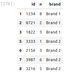
DF# Your code here(Click Here to answer questions)
This is what you should see:
2. Now we need to fix this data - when we read this in there are some weird things happening.
Open the .sales.xlsx file and look in there. Notice that there are two weird rows at the top.
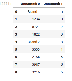
How can we read the data in and skip some rows? Try running the command below to read the documentation. Are there any commands that might help us skip the first three rows when reading in the data?
pd.read_excel?Try writing your own code that will read in the data, skipping three rows, so that it looks like this:
My Answer - you really should try to figure this out without looking!
file_name = 'data/sales.xlsx'
DF = pd.read_excel(file_name,skiprows=3)
DF
3. This is better, but let’s rename the columns
In the lecture above we learned how to rename columns. Rename the columns in this DataFrame so that ‘Unnamed: 0’ becomes ‘id’ and ‘Unnamed: 1’ becomes ‘n’. Your DataFrame should look like
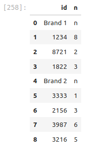
My Answer - you really should be able to figure this out without looking!
DF.rename(columns={'Unnamed: 0':'id','Unnamed: 1':'n'},inplace=True)4. This is better, but….
This is not yet a tidy data frame. Why not?
(Your answer here)
How do we make it tidy?
We need to manipulate the data so that we have three columns. The brand, the id, and then the number of sales, but the brand information is mixed up in the id row. We are going to use the following command:
brand_data = DF['id'].apply(lambda x: x if 'Brand' in str(x) else np.nan)Tell me what each part of this command does. For example break down each piece:
DF[‘id’]
.apply()
lambda x: x if ‘Brand’ in str(x) else np.nan
HINT1 - here you see something new and if else statement.
- The command ‘Brand’ in str(x) will check to see if the word ‘Brand’ is in each row. This will return True or False.
- To test this try DF[‘id’].apply(lambda x: ‘Brand’ in str(x)) in a separate cell.
- The if statement checks to see if ‘Brand’ in str(x) is True. If it is true it returns the x (original data). Otherwise it returns np.nan
- np.nan is how we can get Not a Number.
(Your explanation of the command here)
DF.keys()Index(['religion', 'Less than $30,000', '$30,000-$49,999', '$50,000-$99,999',
'$100,000 or more', 'n'],
dtype='object')# Now just run the command
brand_data = DF['id'].apply(lambda x: x if 'Brand' in str(x) else np.nan)
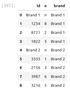
brand_data5. Create a new empty column to store our brand_data
You should know how to add a new column to a data frame. Use the column name ‘brand’.
My Answer - you really should be able to figure this out without looking!
DF['brand'] = brand_data# Your code here6. Lets fill up those NaNs with the brand information
The command .ffill() works like magic! It goes down the column and will fill any NaNs with the information from the cells above, until it gets to another good value. Check out what this command does!
DF=DF.ffill()Your data frame should look like
# Your code here (copy and paste)7. Finally mask out the rows that have bad ‘id’
Create a mask using
mask = DF['id'].apply(lambda x:'Brand' not in str(x) )then apply that mask to get
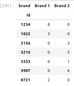
# Your code here7. Now lets pivot!!
Try out the .pivot() command. See if you can create a DataFrame that looks like this:
DF_new.pivot(index=???, columns=???,values=???)
Hint - index=
index=[‘id’]
Hint - columns=
columns=[‘brand’]
Hint - values=
values=‘n’
Hint - change NaN to zero
.fillna(0)
My Answer
DF_piv = DF_new.pivot(index=['id'], columns=['brand'],values=['n']).fillna(0)
DF_piv
# Your code here