import numpy as np
import pandas as pd

import matplotlib.pyplot as plt
import plotly.express as px
from plotly.subplots import make_subplots
import plotly.io as pio
pio.renderers.defaule = 'colab'

from itables import show

# This stops a few warning messages from showing
pd.options.mode.chained_assignment = None
import warnings
warnings.simplefilter(action='ignore', category=FutureWarning)Introduction to Data Science
Introduction to Modeling and Algorithms
Important Information
- Email: joanna_bieri@redlands.edu
- Office Hours: Duke 209 Click Here for Joanna’s Schedule
Announcements
If you are behind it is time to get 100% caught up! I will expect to see you at one of the labs!
Day 15 Assignment - same drill.
- Make sure you can Fork and Clone the Day15 repo from Redlands-DATA101
- Open the file Day15-HW.ipynb and start doing the problems.
- You can do these problems as you follow along with the lecture notes and video.
- Get as far as you can before class.
- Submit what you have so far Commit and Push to Git.
- Take the daily check in quiz on Canvas.
- Come to class with lots of questions!
————————
Today we start venturing into the world of Algorithms and Models. During our ethics week we had lots of discussions about ethical issues with algorithmic bias and decision making using data. Now you are going to get a peak behind the scenes to see how these models are built.
These words are all related!
Mathematical Model – Data Science Prediction – Algorithm – Machine Learning – Artificial Intelligence
What is a Mathematical Model?
A model is used to explain the relationship between variables so that we can make predictions. Ideally we start by doing some exploratory data analysis (EDA) and some basic visualizations to get a feel for our data. Then we start asking some questions like:
- Is there a relationship between A and B?
- If I knew A could I predict B?
This lab follows the Data Science in a Box units “The Language of Models and Fitting and Interpreting Models” by Mine Çetinkaya-Rundel. It has been updated for our class and translated to Python by Joanna Bieri.
Linear vs Nonlinear Models:
A linear model can be described by a straight line.
\[ Y = mX + b \]
Here our goal is to use \(X\) to predict \(Y\). Another example of a linear model is training a machine to make a decision based on crossing a straight line boundary.
Code for creating the linear example graph
# Parameters for the linear relationship
m = 2.5  # slope
b = 5.0  # intercept
num_points = 100  # number of data points
noise_level = 2.0  # standard deviation of noise

# Generate random independent variable (x) values
x = np.random.uniform(0, 10, num_points)

# Generate the dependent variable (y) values using the linear equation
# Adding some random noise (epsilon) to simulate real-world data
epsilon = np.random.normal(0, noise_level, num_points)
y = m * x + b + epsilon
y_nonoise = m * x + b

DF = pd.DataFrame()
DF['x'] = x
DF['y'] = y
DF['yn'] = y_nonoise

DF=DF.sort_values('x')

fig = px.scatter(DF,x='x',y='y')
# Add a line to the plot
fig.add_trace(
    px.line(DF, x='x', y='yn',color_discrete_sequence=['red']).data[0]
)

fig.show()
A nonlinear model cannot be described by a straight line. It might be modeled by a wide range of other functions!
\[ Y = f(X) \]
So that we can use \(X\) to predict \(Y\) and \(f\) is a nonlinear function, or training a machine to make a decision based on crossing a nonlinear boundary.
Code for creating the linear example graph
# Parameters for the nonlinear relationship (quadratic)
a = 1.5  # coefficient for x^2
b = -2.0  # coefficient for x
c = 3.0  # constant term
num_points = 100  # number of data points
noise_level = 1.0  # standard deviation of noise

# Generate random independent variable (x) values
x = np.random.uniform(-2, 2, num_points)

# Generate the dependent variable (y) values using the quadratic equation
# Adding some random noise (epsilon) to simulate real-world data
epsilon = np.random.normal(0, noise_level, num_points)
y = a * x**3 + b * x + c + epsilon
y_nonoise = a * x**3 + b * x + c

DF = pd.DataFrame()
DF['x'] = x
DF['y'] = y
DF['yn'] = y_nonoise

DF=DF.sort_values('x')

fig = px.scatter(DF,x='x',y='y')
# Add a line to the plot
fig.add_trace(
    px.line(DF, x='x', y='yn',color_discrete_sequence=['red']).data[0]
)


fig.show()
Paris Paintings Data
To explore the ideas of modeling data we will use the Paris Paintings dataset.
- Source: Printed catalogs of 28 auction sales in Paris, 1764 - 1780 (Historical Data)
- Data curators Sandra van Ginhoven and Hilary Coe Cronheim (who were PhD students in the Duke Art, Law, and Markets Initiative at the time of putting together this dataset) translated and tabulated the catalogs
- 3393 paintings, their prices, and descriptive details from sales catalogs over 60 variables
They looked at individual catalogs and entered the data by hand. This means that there are some inconsistencies.
n/a vs NA vs empty - all of these should be considered NaN.
Here is an example of what an art auction looks like today. The people at this auction are looking at pamphlets that even include color photos of the painting that is up for sale. Today there are all sorts of ways of getting info about what is up for auction.
In historical times, this was not possible. Instead the information was communicated in printed catalogs without images. This is what the auction of that time might look like.
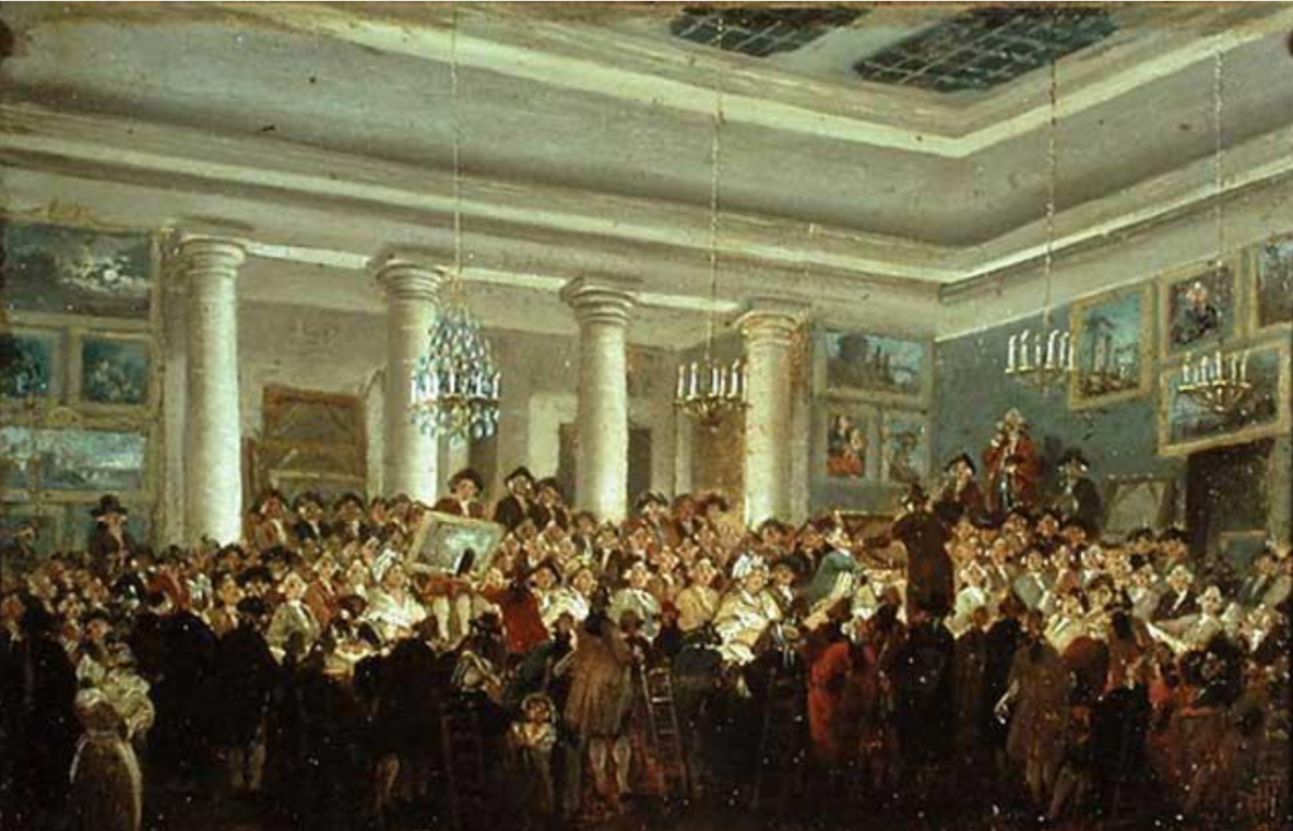
Pierre-Antoine de Machy, Public Sale at the Hôtel Bullion, Musée Carnavalet, Paris (18th century)
The researchers were interested in the Art market. They were students of economics and art history. Their question: Were the auctioneers doing anything to motivate the large increase in sales between the years of 1764-1780?
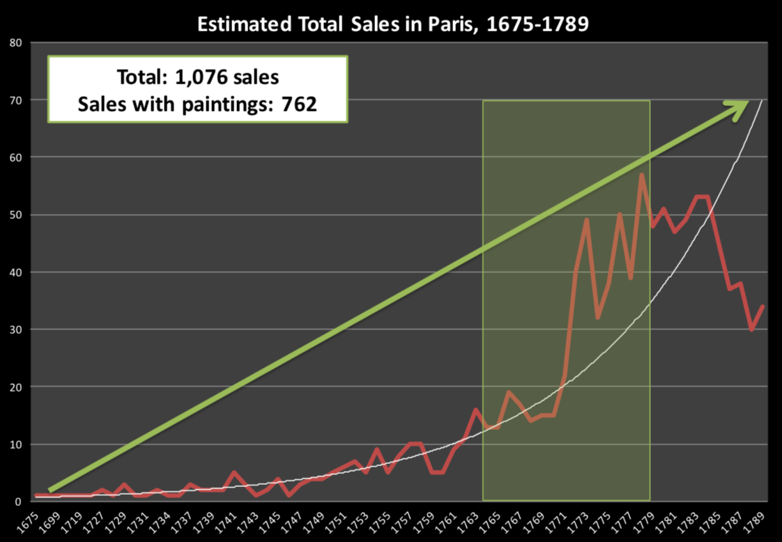
Plot credit: Sandra van Ginhoven
Historical Example
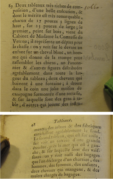
Two paintings very rich in composition, of a beautiful execution, and whose merit is very remarkable, each 17 inches 3 lines high, 23 inches wide; the first, painted on wood, comes from the Cabinet of Madame la Comtesse de Verrue; it represents a departure for the hunt: it shows in the front a child on a white horse, a man who gives the horn to gather the dogs, a falconer and other figures nicely distributed across the width of the painting; two horses drinking from a fountain; on the right in the corner a lovely country house topped by a terrace, on which people are at the table, others who play instruments; trees and fabriques pleasantly enrich the background.
There is data in this description!
Variables in Paris Paintings Data
file_location = 'https://joannabieri.com/introdatascience/data/paris-paintings.csv'
DF_raw_paintings = pd.read_csv(file_location,na_filter=False)show(DF_raw_paintings)| name | sale | lot | position | dealer | year | origin_author | origin_cat | school_pntg | diff_origin | logprice | price | count | subject | authorstandard | artistliving | authorstyle | author | winningbidder | winningbiddertype | endbuyer | Interm | type_intermed | Height_in | Width_in | Surface_Rect | Diam_in | Surface_Rnd | Shape | Surface | material | mat | materialCat | quantity | nfigures | engraved | original | prevcoll | othartist | paired | figures | finished | lrgfont | relig | landsALL | lands_sc | lands_elem | lands_figs | lands_ment | arch | mytho | peasant | othgenre | singlefig | portrait | still_life | discauth | history | allegory | pastorale | other |
|---|---|---|---|---|---|---|---|---|---|---|---|---|---|---|---|---|---|---|---|---|---|---|---|---|---|---|---|---|---|---|---|---|---|---|---|---|---|---|---|---|---|---|---|---|---|---|---|---|---|---|---|---|---|---|---|---|---|---|---|---|
|
Loading ITables v2.1.4 from the internet...
(need help?) |
Lets look at the information for the painting described above.
mask = DF_raw_paintings['name']=='R1777-89a'
show(DF_raw_paintings[mask])| name | sale | lot | position | dealer | year | origin_author | origin_cat | school_pntg | diff_origin | logprice | price | count | subject | authorstandard | artistliving | authorstyle | author | winningbidder | winningbiddertype | endbuyer | Interm | type_intermed | Height_in | Width_in | Surface_Rect | Diam_in | Surface_Rnd | Shape | Surface | material | mat | materialCat | quantity | nfigures | engraved | original | prevcoll | othartist | paired | figures | finished | lrgfont | relig | landsALL | lands_sc | lands_elem | lands_figs | lands_ment | arch | mytho | peasant | othgenre | singlefig | portrait | still_life | discauth | history | allegory | pastorale | other | |
|---|---|---|---|---|---|---|---|---|---|---|---|---|---|---|---|---|---|---|---|---|---|---|---|---|---|---|---|---|---|---|---|---|---|---|---|---|---|---|---|---|---|---|---|---|---|---|---|---|---|---|---|---|---|---|---|---|---|---|---|---|---|
|
Loading ITables v2.1.4 from the internet...
(need help?) |
Some Data Science Questions
- Are any of these variables linearly related?
- Does the size of the paining matter?
- Did the auctioneers do something to drive up sales prices?
- Can we model the prices of the paintings?
- Are higher prices associated with certain features highlighted in the description?
# Make a copy of the data that we can start working on
DF = DF_raw_paintings.copy()

# Do something about all those different NaNs
DF.replace('',np.nan,inplace=True)
DF.replace('n/a',np.nan,inplace=True)
DF.replace('NaN',np.nan,inplace=True)
Modeling - Relationship Between Variables
Is there a linear relationship between the height and width of a painting?
Q Make historgrams of the height and width of all the paintings in the data set. You should be able to recreate the plots below without looking at the code.
# Look at the data types in these columns
my_cols = ['Height_in', 'Width_in']
DF[my_cols].dtypes
Height_in object
Width_in object
dtype: object# Update the types - these should be floats
DF['Height_in'] = DF['Height_in'].apply(lambda x: float(x))
DF['Width_in'] = DF['Width_in'].apply(lambda x: float(x))
DF[my_cols].dtypesHeight_in float64
Width_in float64
dtype: objectHistogram of Height
fig = px.histogram(DF,x='Height_in')

fig.update_layout(template="ggplot2",
                  xaxis_title="Height in inches",
                  yaxis_title="")

fig.show()
Histogram of Width
fig = px.histogram(DF,x='Width_in')

fig.update_layout(template="ggplot2",
                  xaxis_title="Height in inches",
                  yaxis_title="")

fig.show()
Q Explain in words what these plots tell you about the data.
Models as Functions
- We can represent relationships between variables using functions
- A function is a mathematical concept: the relationship between an output and one or more inputs
Plug in the inputs and receive back the output
Example: The formula \[y = 3x + 7\] is a function with input \(x\) and output \(y\).
If \(x\) is \(5\), then \(y\) is \(22\), because \(y = 3 \times (5) + 7 = 22\)
flowchart LR
    A(Inputs) --> B[Function] --> C(Output)
flowchart LR
    A(x=5) --> B[3 * 5 + 7 = 22] --> C(y=22)
Can we find a function that describes the relationship between height and width of painting?
Start by looking at a scatter plot. Is there a relationship at all? Remember we are assuming that the data is somehow linear. That we can model it with a straight line.
Q Make a scatter plot of the width vs the height like the one below. You should be able to recreate the plots here without looking at the code.
Scatterplot Width vs Height
fig = px.scatter(DF,x='Width_in',y="Height_in",color_discrete_sequence=['black'])

fig.update_layout(template="ggplot2",
                  title='Height vs Width of Paris Paintings <br><sup> Paris auctions, 1764-1780</sup>',
                  title_x=0.5,
                  xaxis_title="Width (inches)",
                  yaxis_title="Height (inches)")

fig.show()
Looking at this data there might be a linear relationship. We can add a linear fit line to this plot using the command:
trendline='ols'This uses Ordinary Least Squares fitting to find a reasonable line. We will learn later about how we actually find these lines, but here you will just see you to make them appear in the plot.
fig = px.scatter(DF,
                 x='Width_in',
                 y="Height_in",
                 color_discrete_sequence=['black'],
                trendline='ols',
                trendline_scope='overall',
                trendline_color_override='blue')


fig.update_layout(template="ggplot2",
                  title='Height vs Width of Paris Paintings <br><sup> Paris auctions, 1764-1780</sup>',
                  title_x=0.5,
                  xaxis_title="Width (inches)",
                  yaxis_title="Height (inches)")

fig.show()
results = px.get_trendline_results(fig)
info = results.iloc[0]["px_fit_results"].summary()
print(info) OLS Regression Results
==============================================================================
Dep. Variable: y R-squared: 0.683
Model: OLS Adj. R-squared: 0.683
Method: Least Squares F-statistic: 6749.
Date: Fri, 08 Nov 2024 Prob (F-statistic): 0.00
Time: 10:41:38 Log-Likelihood: -11083.
No. Observations: 3135 AIC: 2.217e+04
Df Residuals: 3133 BIC: 2.218e+04
Df Model: 1
Covariance Type: nonrobust
==============================================================================
coef std err t P>|t| [0.025 0.975]
------------------------------------------------------------------------------
const 3.6214 0.254 14.265 0.000 3.124 4.119
x1 0.7808 0.010 82.150 0.000 0.762 0.799
==============================================================================
Omnibus: 1258.323 Durbin-Watson: 1.707
Prob(Omnibus): 0.000 Jarque-Bera (JB): 27933.347
Skew: 1.375 Prob(JB): 0.00
Kurtosis: 17.363 Cond. No. 45.8
==============================================================================
Notes:
[1] Standard Errors assume that the covariance matrix of the errors is correctly specified.So the line that “fits” this data based on the code we ran is
\[ H = 0.7808 W + 3.6214 \]
Q Where do we think this prediction is most accurate? Where is there the most error? Explain why you think this?
Adding uncertainty to the plot - advanced code
fig = px.scatter(DF,
x='Width_in',
y="Height_in",
color_discrete_sequence=['black'],
trendline='ols',
trendline_scope='overall',
trendline_color_override='blue')
m_se = 0.010
b_se = 0.254
m = 0.7808
b = 3.6214
DF_error = pd.DataFrame()
DF_error['w'] = DF['Width_in']
DF_error['ym'] = (m-m_se)*DF_error['w']+b-b_se
DF_error['yp'] = (m+m_se)*DF_error['w']+b+b_se
DF_error = DF_error.sort_values('w')
# Add a lower uncertainty line
fig.add_trace(
px.line(DF_error, x='w', y='ym',color_discrete_sequence=['lightblue']).data[0]
)
# Add an upper uncertainty line
fig.add_trace(
px.line(DF_error, x='w', y='yp',color_discrete_sequence=['lightblue']).data[0]
)
fig.update_layout(template="ggplot2",
title='Height vs Width of Paris Paintings <br><sup> Paris auctions, 1764-1780</sup>',
title_x=0.5,
xaxis_title="Width (inches)",
yaxis_title="Height (inches)")
fig.show()Did we have to pick this trendline?
No there are other choices:
- ‘ols’: Ordinary Least Squares regression line (linear regression).
- ‘lowess’: Locally Weighted Scatterplot Smoothing (non-linear regression).
- ‘rolling’: Rolling window calculations (e.g., rolling average, rolling median).
- ‘expanding’: Expanding window calculations (e.g., expanding average, expanding sum).
- ‘ewm’: Exponentially Weighted Moving Average (EWMA).
Some of these we will cover in the next few weeks, but some will wait for DATA 201.
Vocab for Modeling
Response variable: Variable whose behavior or variation you are trying to understand, on the y-axis
Explanatory variables: Other variables that you want to use to explain the variation in the response, on the x-axis
Predicted value: Output of the model function
- The model function gives the typical (expected) value of the response variable conditioning on the explanatory variables
Residuals: A measure of how far each case is from its predicted value (based on a particular model)
- Residual = Observed value - Predicted value
- Tells how far above/below the expected value each case is
Adding residual color to the plot - advanced code
# Add some conditional coloring - advanced Python list comprehension
DF['residual_hw'] = ['Positive residual' if H > 0.7808*W + 3.6214 else 'Negative residual' for H,W in zip(DF['Height_in'],DF['Width_in']) ]
fig = px.scatter(DF,
x='Width_in',
y="Height_in",
color='residual_hw',
color_discrete_sequence=['purple','black'],
trendline='ols',
trendline_scope='overall',
trendline_color_override='blue')
fig.update_layout(template="ggplot2",
title='Height vs Width of Paris Paintings <br><sup> Paris auctions, 1764-1780</sup>',
title_x=0.5,
xaxis_title="Width (inches)",
yaxis_title="Height (inches)",
legend_title = '')
fig.show()Investigate the clustering of points
When creating scatter plots, sometimes it is hard to see when there are lots of points on top of each other. Changing the opacity (or alpha value) can help! This will make the points in the plot more transparent.
Scatterplot Width vs Height - Opacity=0.2
fig = px.scatter(DF,
x='Width_in',
y="Height_in",
color_discrete_sequence=['black'],
opacity=0.2)
fig.update_layout(template="ggplot2",
title='Height vs Width of Paris Paintings <br><sup> Paris auctions, 1764-1780</sup>',
title_x=0.5,
xaxis_title="Width (inches)",
yaxis_title="Height (inches)")
fig.show()What starts to be apparent?
- We see a V in the plot!
- How many straight lines would you draw to model this data?
- What is going on here?
Painting types
- Landscape painting is the depiction in art of landscapes – natural scenery such as mountains, valleys, trees, rivers, and forests, especially where the main subject is a wide view – with its elements arranged into a coherent composition.
- Landscape paintings tend to be wider than they are long.
- Portrait painting is a genre in painting, where the intent is to depict a human subject.
- Portrait paintings tend to be longer than they are wide.
Source: Wikipedia, Landscape painting
Source: Wikipedia, Portait painting
# Look at the landscape data
DF['landsALL'].value_counts().rename_axis('Landscape').reset_index(name='Counts')| Landscape | Counts | |
|---|---|---|
| 0 | 0 | 2119 |
| 1 | 1 | 1274 |
# We want to think of this as categorical!
# 0 = not landscape, 1= landscape
# One way to do this is to turn the data into a string
DF['landsALL'] = DF['landsALL'].apply(lambda x: str(x))Scatterplot Width vs Height - Opacity=0.2
fig = px.scatter(DF,
x='Width_in',
y="Height_in",
color='landsALL',
opacity=0.2,
trendline='ols')
fig.update_layout(template="ggplot2",
title='Height vs Width of Paris Paintings <br><sup> Paris auctions, 1764-1780</sup>',
title_x=0.5,
xaxis_title="Width (inches)",
yaxis_title="Height (inches)")
fig.show()We added another variable by coloring by whether or not there were landscape features in the painting. Then the trendline=‘ols’ now gives us two lines. Here there is some evidence that if a painting in landscape, then it tends to be wider than it is tall.
Why is one line shorter? We could extend this line this is called extrapolation. Be very careful with this because extrapolation can cause a lot of uncertainty. We really don’t have enough data to confidently extend this line.
If we wanted to look at the data for two trendlines we would run:
results = px.get_trendline_results(fig)
info = results.iloc[0]["px_fit_results"].summary()
print(info)
results = px.get_trendline_results(fig)
info = results.iloc[1]["px_fit_results"].summary()
print(info)Models - upsides and downsides
- Models can sometimes reveal patterns that are not evident in a graph of the data. This is a great advantage of modeling over simple visual inspection of data.
- There is a real risk, however, that a model is imposing structure that is not really there on the scatter of data, just as people imagine animal shapes in the stars. A skeptical approach is always warranted.
- Just because you fit a model does not mean you found a true relationship.
Variation around the model.
Variation or Uncertainty is just as important as the model, if not more!
Statistics is the explanation of variation in the context of what remains unexplained.
- The scatter suggests that there might be other factors that account for large parts of painting-to-painting variability, or perhaps just that randomness plays a big role.
- Adding more explanatory variables to a model can sometimes usefully reduce the size of the scatter around the model.
How do we use models?
TWO MAIN USES:
- Explanation: Characterize the relationship between \(y\) and \(x\) via slopes for numerical explanatory variables or differences for categorical explanatory variables
- Prediction: Plug in \(x\), get the predicted \(y\)
Exercise 1 Redo the plot above except color by some other variable that takes values of zero or one. Describe what the ols trendline tells you about the height and width of that type of painting. Eg. Does a painting being described as pastoral mean it is taller or wider than if it is not pastoral?
- Choose a column that has just 0 and 1 as entries
- Change those values into strings using apply and lambda
- Do a value counts and talk about the balance in the data
- Create a scatter plot with an old trendline colored by your focal column
- Describe in words what you plot is telling you.
————————
Predicting the Height of a Painting given the Width - Regression
Now we are ready to build a model for our paintings using Python Machine Learning. We will assume a linear model.
\[ height_i = \beta_1 width_i + \beta_0 \]
We need to install some really powerful packages to help us with modeling and machine learning.
Scikit-Learn
Scikit Learn: https://scikit-learn.org/stable/
!conda install -y scikit-learnLinear (Least Squares) Regression - Supervised Machine Learning
In a simple two variable case we can actually just solve for the slope and intercept using the properties of linear regression:
- The regression line goes through the center of mass point, the coordinates corresponding to average \(x\) and average \(y\), \((\bar{x}, \bar{y})\):
\[\bar{y} = b_0 + b_1 \bar{x} ~ \rightarrow ~ b_0 = \bar{y} - b_1 \bar{x}\]
- The slope has the same sign as the correlation coefficient: \(b_1 = r \frac{s_y}{s_x}\)
- The sum of the residuals is zero: \(\sum_{i = 1}^n e_i = 0\)
- The residuals and \(x\) values are uncorrelated
In general the linear regression computation works by assuming there exists a straight line that can predict our data. The process for finding this line needs some more advanced mathematics but here is the idea for our example:
- Choose a straight line \(\hat{y}_i=b_0 + b_1 x_i\) - here \(b_0\) and \(b_1\) are things we hope to learn from our sample statistics.
- See how well that line fits the sample data by calculating the error or cost or mean squared error \[cost = \frac{1}{n}\sum_{i=1}^n (y_i-\hat{y}_i)^2 \] where \(y_i\) is the value from our sample data and \(\hat{y}_i\) is the value predicted from our model.
- We want this cost to be small so that all of the model predictions are as close as possible to our data. The cost can’t be zero unless our data is in a straight line.
- We change \(b_0\) and \(b_1\) using something called gradient descent to learn what the best possible \(b\) values are.
- Once we can’t make our cost any smaller we stop.
Train a Linear Regression Model
This happens in three steps
- Data Preprocessing
- Model Training
- Analyze the output - predictions
# A new package import!
from sklearn.linear_model import LinearRegression
Preprocessing the Data
Before you can build a model you need to do some cleaning and preprocessing of your data. Here are some important steps:
- Select the variables that you wan to use (columns)
- Decide what to do about NaNs or other strange data
- (advanced) Think about rescaling and standardizing
- Create the inputs and outputs (sometimes encode)
- (advanced) Test - Train split
# Select the variables - I want to predict height given width
DF_model = DF[['Height_in','Width_in']]
DF_model.dtypes
Height_in float64
Width_in float64
dtype: object# Check out the NaNs
# How many Nans
print('Number of NaNs:')
print(DF_model.isna().sum().sum())
print('----------------------')
# What percent of the data is this?
print('Percent NaNs:')
print(DF_model.isna().sum().sum()/len(DF))
print('----------------------')
# I am going to drop these! This is a choice!
DF_model.dropna(inplace=True)
print('Number of NaNs after drop:')
print(DF_model.isna().sum().sum())
print('----------------------')Number of NaNs:
508
----------------------
Percent NaNs:
0.14972001178897731
----------------------
Number of NaNs after drop:
0
----------------------# Create the inputs X (explanatory variable) and the outputs y (response variable)
# .values just gets the numbers that we need
# .reshape(-1,1) puts the X data in the right shape.
X = DF_model['Width_in'].values.reshape(-1, 1)
y = DF_model['Height_in'].valuesTrain the model
- Create the base model, in this case LinearRegression()
- Train the model using the training data
- Look at the results.
# Create linear regression object - a random straight line
LM = LinearRegression()

# Train the model using the data
LM.fit(X, y)LinearRegression()In a Jupyter environment, please rerun this cell to show the HTML representation or trust the notebook.
On GitHub, the HTML representation is unable to render, please try loading this page with nbviewer.org.
LinearRegression()
# The coefficient is the slope
LM.coef_array([0.78079641])# We can also see the intercept
LM.intercept_3.6214055418381896This means that linear regression found the line
\[ height_i = 3.6214055418381896 + 0.78079641 * width_i \]
so given a width we could predict a height. There appears to be a positive relationship between height and width - in general as the width increases the height increases.
Now we can use our model to make a prediction
Let’s say we know a painting had certain width, we can predict the height
width = 33
width = np.array(width).reshape(-1,1)
LM.predict(width)array([29.38768703])width = 0
width = np.array(width).reshape(-1,1)
LM.predict(width)array([3.62140554])Slope: For each additional inch the painting is wider, the height is expected to be higher, on average, by 0.781 inches.
Intercept: Paintings that are 0 inches wide are expected to be 3.62 inches high, on average. (Does this make sense?)
Correlation does not imply causation

Source: XKCD, Cell phones
fig = px.scatter(DF,
                 x='Width_in',
                 y="Height_in",
                 color_discrete_sequence=['black'],
                 opacity=0.2)

fig.update_layout(template="ggplot2",
                  title='Height vs Width of Paris Paintings <br><sup> Paris auctions, 1764-1780</sup>',
                  title_x=0.5,
                  xaxis_title="Width (inches)",
                  yaxis_title="Height (inches)")

# Add the line our model would predict
DF_model = pd.DataFrame()
DF_model['w'] = DF['Width_in']
DF_model['y'] = LM.coef_*DF_model['w']+LM.intercept_
DF_model = DF_model.sort_values('w')

fig.add_trace(
    px.line(DF_model, x='w', y='y',color_discrete_sequence=['blue']).data[0]
)

fig.show()
Check the accuracy of your model
LM.score() uses the R^2 score:
The R2 score is calculated using the formula \[R^{2}=1-\frac{RSS}{TSS}\], where:
- \(R^{2}\) is the coefficient of determination - \(RSS\) is the sum of squares of residuals - \(TSS\) is the total sum of squares
Here’s what the \(R^2\) score means: - \(R^2\) = 0 The model is not able to predict the outcome any better than using the average value. There is no linear relationship between the variables. - \(R^2\) between 0 and 1 The model can partially predict the outcome, but the estimates are not perfect. - \(R^2\) = 1 The model can perfectly predict the outcome. All points lie exactly on a straight line.
NOTE In a true machine learning workflow you would first separate your data into training and testing sets, so you have some data that your model never saw during training. Then you can see how accurate it is on the testing set after training is complete.
LM.score(X, y)0.6829467672722757Exercise 2 Redo the analysis to see if you can use the size (‘Surface’) of the painting to predict the price.
Create a data frame with only the price and surface columns
Look at the data types
Preprocess the data - remove NaNs and change the Surface values to floats.
Train a linear regression model that takes as an input X = Surface Area and gives as an output y=price
    X = DF_model['Surface'].values.reshape(-1,1)
    y = DF_model['price'].values
Plot a scatter plot of Price vs Surface add in your predicted line
Look at the score
Interpret your results. Should you use a linear model to predict the price of a painting using the surface area?
Below you can see the scatter plot and score that I got.
# The score from my model
LM.score(X,y)0.011141075251450694What about Categorical Data?
We can use categorical data as our explanatory variable in Linear Regression but this adds one more step to the process. Whenever we are doing linear regression we are trying to find an equation like
\[ \hat{y} = b_0 + b_1 x \]
But what if x has categorical values? For example does the price of a painting depend on whether or not it was landscape?
x = “landscape” or “not landscape”
y = height of painting.
The equation
\[ \hat{y} = b_0 + b_1 landscape \]
does not make sense. So we need to turn the categorical data into a number somehow. In our case we see that we have zeros and ones saved as strings in the ‘landsALL’ column. This means that
0 = “not landscape” 1 = “landscape”
# Change those strings back into ints
DF['landsALL'] = DF['landsALL'].apply(lambda x: int(x))
# Select the variables - I want to predict height given width
DF_model = DF[['landsALL','Height_in']]
DF_model.dtypeslandsALL int64
Height_in float64
dtype: object# Check out the NaNs
# How many Nans
print('Number of NaNs:')
print(DF_model.isna().sum().sum())
print('----------------------')
# What percent of the data is this?
print('Percent NaNs:')
print(DF_model.isna().sum().sum()/len(DF))
print('----------------------')
# I am going to drop these! This is a choice!
DF_model.dropna(inplace=True)
print('Number of NaNs after drop:')
print(DF_model.isna().sum().sum())
print('----------------------')Number of NaNs:
252
----------------------
Percent NaNs:
0.07427055702917772
----------------------
Number of NaNs after drop:
0
----------------------# Create the inputs X (explanatory variable) and the outputs y (response variable)
X = DF_model['landsALL'].values.reshape(-1,1)
y = DF_model['Height_in'].values# Create linear regression object - a random straight line
LM = LinearRegression()
# Train the model using the data
LM.fit(X, y)LinearRegression()In a Jupyter environment, please rerun this cell to show the HTML representation or trust the notebook.
On GitHub, the HTML representation is unable to render, please try loading this page with nbviewer.org.
LinearRegression()
print(LM.coef_)
print(LM.intercept_)[-5.64512764]
22.67991790661878How do we interpret this result?
\[ Height = 22.68 - 5.65 (landsALL) \]
So if landsALL = 0 (not a landscape) the paintings have an average height of 22.68. If landsALL = 1 (it is a landscape) then the height on average is reduced by 5.65 inches. We found that landscapes tend to be shorter.
More than two categories - One Hot Encoding
In the case above we could easily code the categorical to just be 0 or 1. Because there were only two options. If there are more than two options we have to choose a way to encode the data. There is more than one way to do this. We will do something called one-hot encoding
How doe the school of the painting effect the price?
(A = Austrian, D/FL = Dutch/Flemish, F = French, G = German, I = Italian, S = Spanish, X = Unknown)
from sklearn.preprocessing import OneHotEncodermy_columns = ['school_pntg','price']
DF_model = DF[my_columns]
DF_model| school_pntg | price | |
|---|---|---|
| 0 | F | 360.0 |
| 1 | I | 6.0 |
| 2 | D/FL | 12.0 |
| 3 | F | 6.0 |
| 4 | F | 6.0 |
| ... | ... | ... |
| 3388 | F | 18.0 |
| 3389 | F | 25.0 |
| 3390 | F | 80.0 |
| 3391 | F | 5.0 |
| 3392 | F | 5.0 |
3393 rows × 2 columns
DF_model['school_pntg'].value_counts()school_pntg
D/FL 1492
F 1386
I 428
X 69
G 9
S 7
A 2
Name: count, dtype: int64# Get the data we want to predict
X = DF_model['school_pntg'].values.reshape(-1,1)
y = DF_model['price'].values
# Now because X has lots of categories, we need to encode it:
encoder = OneHotEncoder()
X = encoder.fit_transform(X)What does the encoded data look like?
The encoded data puts a one in a location representing each category in the data
['A', 'D/FL', 'F', 'G', 'I', 'S', 'X']so
[1,0,0,0,0,0,0] = AHere is code to look at the categories:
categories = encoder.categories_[0]
categoriesarray(['A', 'D/FL', 'F', 'G', 'I', 'S', 'X'], dtype=object)# Look at each category and encoding
result = DF_model.groupby('school_pntg',as_index=False).first()
encoded_data = encoder.transform(result['school_pntg'].values.reshape(-1,1))
for i,e in enumerate(encoded_data.toarray()):
print(categories[i])
print(e)
print('---------------------------')A
[1. 0. 0. 0. 0. 0. 0.]
---------------------------
D/FL
[0. 1. 0. 0. 0. 0. 0.]
---------------------------
F
[0. 0. 1. 0. 0. 0. 0.]
---------------------------
G
[0. 0. 0. 1. 0. 0. 0.]
---------------------------
I
[0. 0. 0. 0. 1. 0. 0.]
---------------------------
S
[0. 0. 0. 0. 0. 1. 0.]
---------------------------
X
[0. 0. 0. 0. 0. 0. 1.]
---------------------------Now we can train the linear regression just like we did above
# Create linear regression object - a random straight line
LM = LinearRegression()

# Train the model using the data
LM.fit(X, y)
# Look at the information we get
print(LM.coef_)
print('------------------------------')
print(LM.intercept_)[-607.0226627 462.24135005 -265.17807213 -650.46710718 -304.23294435
2045.54876584 -680.88932952]
------------------------------
715.0226600517791What the heck does this mean?!?!?
Well the output coeficients line up with the labels:
| Label | Coef |
|---|---|
| A | -607.0226627 |
| D/FL | 462.24135005 |
| F | -265.17807213 |
| G | -650.46710718 |
| I | -304.23294435 |
| S | 2045.54876584 |
| X | -680.88932952 |
We we can interpret this as the average base cost of a painting was about 715.02, but if the painting was Austrian then on average it sold from 607.02 less but if it was Spanish then on average it sold for 2045.55 more. The equation looks something like this:
\[ Price = 715.02 + -607.0226627(A) + 462.24135005*(D/FL) -265.17807213(F) -650.46710718(G) -304.23294435(I) + 2045.54876584(S) - 680.88932952(X)\]
Where only one of these can be equal to one at a time, all others are zero.
Exercise 3 Redo the analysis above except this time see if the school of the painting effects the overall size (‘Surface’) of the painting. Don’t forget to drop the NaNs where we don’t know the surface size and change the surface variables to floats.
Create a data frame with only the school and surface columns
Look at the data types
Preprocess the data - remove NaNs and change the Surface values to floats.
Train a linear regression model that takes as an input X = School and gives as an output y= surface area, now you need to one hot encode the X values!
    X = DF_model['school_pntg'].values.reshape(-1,1)
    y = DF_model['Surface'].values
Look at the output, what does it mean? - Which school of paintings on average are largest? smallest?
You can see the outputs of my code below.
['A' 'D/FL' 'F' 'G' 'I' 'S' 'X']
------------------------------
[-392.07405544 -266.70347449  122.28771743 -393.21155591  142.65081971
 1051.64022987 -264.58968117]
------------------------------
686.0740419935794