Blue Q boxes are questions for you to answer by hand, in a notebook, with a pen. Not because I am old fashioned. Writing something down by hand is slow, and slow is the point: it is very hard to write an explanation you do not actually understand. You are welcome to use AI in this class for the mechanics of code, but these boxes are the part where you do the thinking yourself. Bring your written notes to class, I will ask to see them.
Green You Try boxes are optional code for you to work through. Nothing is collected and nothing is graded. They are there because you will learn more from changing a number and rerunning than from watching me do it.
Every code cell begins with a tag that tells you what to do with it.
# RUN THIS. Setup, loading data, a plot. Copy it, run it, move on. You do not need to be able to write it from memory.
# LEARN TO WRITE THIS. The pattern of the day. The homework will ask you for it, and so will the exam. Type it out yourself at least once rather than pasting it.
# DEMO ONLY. Code that exists to show one idea. You do not need to be able to write it yourself.
# UNDERSTAND THESE STEPS. Code that shows how something works inside, one small step at a time. Read it and make sure you understand what each line does. You do not need to memorize it or be able to write it from scratch.
Reading: Geron chapter 10, the sections Implementing a Regression MLP and Implementing Mini-Batch Gradient Descent using DataLoaders.
Last class we built one neuron by hand and taught it with gradient descent. The loop had five steps: predict, loss, backward, update, clear. Today we do three new things with that loop.
More neurons. We put neurons side by side in a layer, and stack layers into a multilayer perceptron (MLP), which is the simplest kind of neural network.
PyTorch’s tools. PyTorch has ready made pieces for the layers, the loss and the update step, so we do not have to write every weight by hand.
Mini-batches. Instead of using every row for every step, we use a small batch of rows at a time. This is how almost every neural network is trained.
Today’s problem is regression: we predict a number instead of a yes or no. The data is the California housing data from the reading.
Here is the plan for today:
Fit a linear regression, so we have a number to beat.
Build a layer of neurons and then an MLP.
Train the MLP with PyTorch’s loss and optimizer, using all the rows at every step.
Train it again with mini-batches, and compare.
The California Housing Data
Each row is one small neighborhood (a census block group) in California in 1990. The label is the median house value in the neighborhood, in units of $100,000, so 2.5 means $250,000.
column
what it means
MedInc
median income in the neighborhood (in units of $10,000)
HouseAge
median age of the houses
AveRooms
average number of rooms per household
AveBedrms
average number of bedrooms per household
Population
number of people in the neighborhood
AveOccup
average number of people per household
Latitude, Longitude
where the neighborhood is
MedHouseVal
median house value, in units of $100,000. This is what we predict.
# RUN THIS. Imports and the data.import numpy as npimport pandas as pdimport matplotlib.pyplot as plthousing = pd.read_csv("data/california_housing.csv")print("rows and columns:", housing.shape)print("missing values:", housing.isna().sum().sum())
rows and columns: (20640, 9)
missing values: 0
housing.head()
MedInc
HouseAge
AveRooms
AveBedrms
Population
AveOccup
Latitude
Longitude
MedHouseVal
0
8.3252
41.0
6.984127
1.023810
322.0
2.555556
37.88
-122.23
4.526
1
8.3014
21.0
6.238137
0.971880
2401.0
2.109842
37.86
-122.22
3.585
2
7.2574
52.0
8.288136
1.073446
496.0
2.802260
37.85
-122.24
3.521
3
5.6431
52.0
5.817352
1.073059
558.0
2.547945
37.85
-122.25
3.413
4
3.8462
52.0
6.281853
1.081081
565.0
2.181467
37.85
-122.25
3.422
Just like what we did last class, we are not choosing a final model today. We are learning how to train a network, so we use a training set and a validation set and there is no test set. We scale the features because neural networks need scaled features, just like logistic regression did.
# RUN THIS. Features, label, split, scale.from sklearn.model_selection import train_test_splitfrom sklearn.preprocessing import StandardScalerfrom sklearn.pipeline import PipelineX = housing.drop(columns=["MedHouseVal"])y = housing["MedHouseVal"]X_train, X_valid, y_train, y_valid = train_test_split( X, y, test_size=0.25, random_state=42)# The preprocessing pipeline. Today it is only a scaler, but we still# put it in a pipeline so our code looks the same every time.preprocessing = Pipeline([ ("scale", StandardScaler())])# fit_transform on the training data: learn the mean and std from the training rowsX_train_scaled = preprocessing.fit_transform(X_train)# transform only on the validation data: reuse the training mean and stdX_valid_scaled = preprocessing.transform(X_valid)print("training rows:", X_train_scaled.shape)print("validation rows:", X_valid_scaled.shape)
training rows: (15480, 8)
validation rows: (5160, 8)
A number to beat - old fashioned Linear Regression
Before we build anything new, let’s see how a plain linear regression does. We measure every model today with the RMSE (root mean squared error). It is in the same units as the label, so an RMSE of 0.5 means the predictions are typically off by about $50,000.
# LEARN TO WRITE THIS. The baseline.from sklearn.linear_model import LinearRegressionfrom sklearn.metrics import root_mean_squared_error# A scikit-learn model goes in a full pipeline: the preprocessing and the model togetherlin_pipeline = Pipeline([ ("prep", preprocessing), # the same preprocessing as above ("model", LinearRegression())])lin_pipeline.fit(X_train, y_train) # the raw rows, the pipeline scales them for usy_pred_lin = lin_pipeline.predict(X_valid)rmse_lin = root_mean_squared_error(y_valid, y_pred_lin)print("linear regression validation RMSE:", round(rmse_lin, 4))
linear regression validation RMSE: 0.7356
So a straight line is typically off by about $73,600. Can a neural network do better?
When can I use a pipeline?
From now on we follow two rules:
A scikit-learn model always goes in a full Pipeline: the preprocessing and the model together, fit once on the raw training rows. That is what we did for the baseline above.
A PyTorch model can not go inside a scikit-learn Pipeline, because it does not have .fit() and .predict(). We still build the preprocessing as a pipeline, fit it on the training rows only, and hand its output to PyTorch. That is what X_train_scaled and X_valid_scaled are.
Either way the preprocessing learns from the training rows only, so there is no leakage. Today the preprocessing is only a scaler, but in the weekly homework it also fills in missing values and makes dummy columns, and the pattern is exactly the same.
From One Neuron to a Layer
First we turn the data into tensors, just like last class.
Then PyTorch wants the labels (y-data) as a column, with one row per house and one number in each row. That is what .reshape(-1, 1) does. Shape mismatch errors are the most common error when putting together a multilayer networks.
# LEARN TO WRITE THIS. The data as tensors.import torchX_train_t = torch.tensor(X_train_scaled, dtype=torch.float32)X_valid_t = torch.tensor(X_valid_scaled, dtype=torch.float32)y_train_t = torch.tensor(y_train.values, dtype=torch.float32).reshape(-1, 1) # -1 means "choose the size from the data", 1 means one columny_valid_t = torch.tensor(y_valid.values, dtype=torch.float32).reshape(-1, 1)print("X_train_t:", X_train_t.shape)print("y_train_t:", y_train_t.shape)
Last class we made the weights by hand with the command torch.zeros(11, requires_grad=True). PyTorch has a tool that does this for us: nn.Linear. It does all of the things: stores the weights and the bias, tracks them for autograd, and computes the weighted sum.
nn.Linear(8, 1) is one neuron with 8 inputs. It is exactly the weighted sum from last class, without the sigmoid.
# LEARN TO WRITE THIS. One neuron, the PyTorch way.import torch.nn as nntorch.manual_seed(42) # so everyone starts with the same random weightsone_neuron = nn.Linear(8, 1) # 8 inputs, 1 outputprint("weights:", one_neuron.weight)print("bias:", one_neuron.bias)
Notice that the weights do not start at zero. nn.Linear starts them at small random numbers. We will see why that matters later… but you can guess it has something to do with gradients!
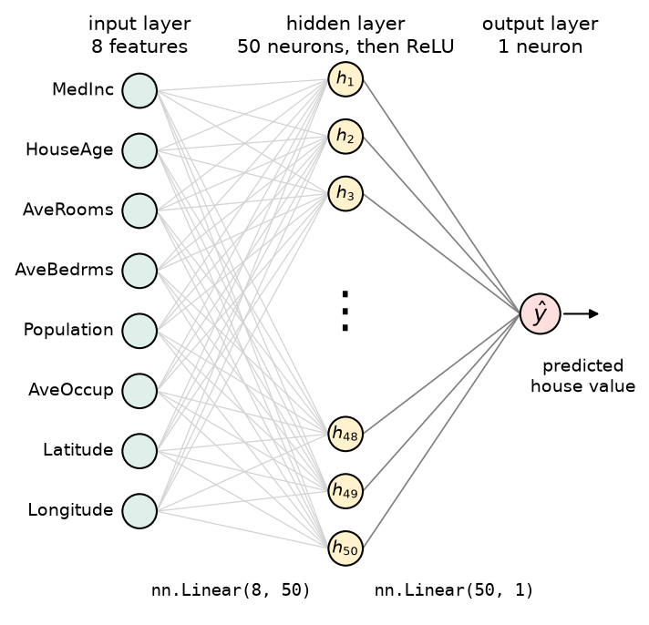
We can do much more complicated things. For example we can add more neurons! nn.Linear(8, 50) is 50 neurons side by side, which is called a layer. Each of the 50 neurons gets all 8 inputs and has its own 8 weights and its own bias. So one row of data goes in, and 50 numbers come out, one from each neuron.
Here is a picture of that layer, along with the one output neuron we add in the next section:
Our MLP. The 8 features on the left each connect to every one of the 50 hidden neurons in the middle, and all 50 hidden neurons connect to the one output neuron on the right.
Every line in the picture is one weight. Each of the 8 features on the left connects to every hidden neuron, and each hidden neuron also has its own bias. We only drew 6 of the 50 hidden neurons, the dots stand for the rest.
# LEARN TO WRITE THIS. A layer of 50 neurons.layer = nn.Linear(8, 50)# Look at the sizesprint("weights:", layer.weight.shape) # 50 neurons, 8 weights eachprint("biases:", layer.bias.shape) # one bias per neuron# Put five houses each with 8 variables into the neuronprint("input shape for 5 houses:", X_train_t[:5].shape)out = layer(X_train_t[:5]) # Get out 50 variables/results for each of the 5 houses.print("output for 5 houses:", out.shape)
weights: torch.Size([50, 8])
biases: torch.Size([50])
input shape for 5 houses: torch.Size([5, 8])
output for 5 houses: torch.Size([5, 50])
NoteQ1. Write this one out by hand
a. How many weights and how many biases are in nn.Linear(8, 50)? How many numbers is that in total?
b. Last class the neuron ended with a sigmoid. Why would a sigmoid at the end be a bad idea for predicting house values?
A Multilayer Perceptron
A multilayer perceptron (MLP) stacks layers. The outputs of one layer become the inputs of the next layer. Our first MLP has two layers:
A hidden layer of 50 neurons. It is called hidden because we never see its outputs directly.
An output layer of 1 neuron, which takes the 50 numbers from the hidden layer and gives one prediction.
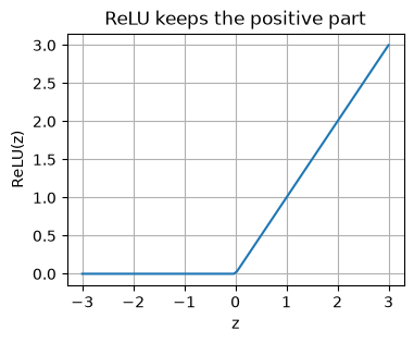
Between them goes an activation function. Today we use ReLU (rectified linear unit), which keeps positive numbers and turns negative numbers into 0:
\text{ReLU}(z) = \max(0, z)
This is not the only possible activation function for regression, we will talk about more in a later class. Here is what the ReLU looks like:
# DEMO ONLY. What ReLU looks like.z = torch.linspace(-3, 3, 100)plt.figure(figsize=(4, 3))plt.plot(z, torch.relu(z))plt.xlabel("z")plt.ylabel("ReLU(z)")plt.title("ReLU keeps the positive part")plt.grid()plt.show()
Why do we need the activation in the middle? If we stack two linear layers with nothing between them, the result is still a straight line. A weighted sum of weighted sums is just another weighted sum. ReLU adds a nonlinearity, and that nonlinearity is what lets the network learn patterns that are not straight lines.
An example: two layers with no activation
Let’s see this with small layers. Say the first layer is nn.Linear(3, 4): 3 inputs and 4 neurons. It holds a 4 by 3 matrix of weights W_1 and 4 biases b_1, and it computes
h = W_1 x + b_1
The second layer is nn.Linear(4, 1): 4 inputs and 1 neuron. It holds a 1 by 4 matrix of weights W_2 and one bias b_2, and it computes
\hat{y} = W_2 h + b_2
Now put the first equation into the second and multiply it out:
\hat{y} = W_2 (W_1 x + b_1) + b_2 = (W_2 W_1) x + (W_2 b_1 + b_2)
W_2 W_1 is a 1 by 3 matrix and W_2 b_1 + b_2 is one number. So the two layers together are exactly onenn.Linear(3, 1), with weights W = W_2 W_1 and bias b = W_2 b_1 + b_2. The four extra neurons in the middle did not add anything!
Let’s check it with code.
# DEMO ONLY. Two linear layers with nothing between them are one linear layer.torch.manual_seed(42)layer1 = nn.Linear(3, 4)layer2 = nn.Linear(4, 1)# gather the weights and biases into one layer, using the math aboveW = layer2.weight @ layer1.weight # (1 by 4) times (4 by 3) gives 1 by 3b = layer2.weight @ layer1.bias + layer2.bias # one numberx = torch.tensor([[1.0, 2.0, 3.0], [0.5, -1.0, 2.0]]) # two made up rows with 3 features eachwith torch.no_grad():print("two layers: ", layer2(layer1(x)).flatten())print("one layer W, b: ", (x @ W.T + b).flatten())print("with ReLU between:", layer2(torch.relu(layer1(x))).flatten())print()print("the 4 hidden values for each row:")print(layer1(x))
two layers:       tensor([-0.0399, -0.4823])
one layer W, b:   tensor([-0.0399, -0.4823])
with ReLU between: tensor([-0.0399, -0.3691])

the 4 hidden values for each row:
tensor([[ 1.4206,  0.7051,  2.2023,  0.8228],
        [-0.1025,  0.7029,  0.8167, -0.5790]])
The two layers and the one combined layer give exactly the same answers. With ReLU in between, the first row does not change but the second row does.
Look at the hidden values: for the first row all four are positive, so ReLU leaves them alone. The second row has two negative hidden values, ReLU turns them into 0, and that changes the answer. That is the nonlinearity being applied, and it is what lets stacked layers learn things one linear layer can not.
Now how do we stack the layers?
nn.Sequential puts the pieces in order. Data goes in the top and comes out the bottom.
Here we have our 8 input variables mapping through linear functions to 50 hidden neurons, those all go through the nonlinear ReLU, and then the 50 neurons are mapped to 1 output. We want just one prediction (house price) so that last layer should be only one neuron.
# RUN THIS. HOW MANY PARAMETERS DO WE NEED TO LEARN?!?n_params =0for p in model.parameters(): # model.parameters() gives every weight and bias tensor n_params = n_params + p.numel() # numel() is the number of numbers in the tensorprint("numbers to learn:", n_params)
numbers to learn: 501
NoteQ2. Write this one out by hand
a. Show where the 501 comes from. Count the weights and biases in each layer.
b. Why do we need nn.ReLU() between the two layers? What would the model be without it? Give your own example
Training the MLP with PyTorch’s Tools
Last class we wrote the gradient update and the clearing by hand. PyTorch has two tools that do this for us.
A loss function. For regression we use the mean squared error, nn.MSELoss().
An optimizer. torch.optim.SGD (stochastic gradient descent) does the update step for every weight in the model. We give it model.parameters() so it knows which numbers to update, and a learning rate. NOTE: Stochastic means random. In stochastic gradient descent the randomness comes from using a random batch of rows at each step, which we do in the Mini-Batches section below. When we use every row at every step, SGD is just plain gradient descent.
Here is how last class’s five steps line up with today’s code:
Last Class
Today
p = torch.sigmoid(X @ w + b)
y_pred = model(X_train_t)
loss = F.binary_cross_entropy(p, y)
loss = loss_fn(y_pred, y_train_t)
loss.backward()
loss.backward()
w -= learning_rate * w.grad (and the same for b)
optimizer.step()
w.grad.zero_() (and the same for b)
optimizer.zero_grad()
NOTE - We call optimizer.zero_grad() at the start of each step instead of the end. It does the same job, it just makes sure the gradients are clear before we compute new ones.
First we use all of the training rows at every step, like last class.
# LEARN TO WRITE THIS. The training loop, using every row at every step.# Create the seed so the results are repeatabletorch.manual_seed(42)# Create the model - this is where you define your networkmodel = nn.Sequential( nn.Linear(8, 50), nn.ReLU(), nn.Linear(50, 1))# Define your loss function# There are lots of possible loss functions in the torch.nn package# We will use Mean Squared Errorloss_fn = nn.MSELoss()# Define your gradient descent = optimizeroptimizer = torch.optim.SGD( model.parameters(), # the numbers the optimizer is allowed to change lr=0.1) # lr is the learning rate# Decide how many training steps you want to taken_steps =1000for step inrange(n_steps): optimizer.zero_grad() # 1. clear the old gradients y_pred = model(X_train_t) # 2. predict - run the data through the model loss = loss_fn(y_pred, y_train_t) # 3. loss - calculate the error loss.backward() # 4. backward - get the gradients "back propagation" optimizer.step() # 5. update every weight and biasif step %200==0: # print every 200 stepsprint("step", step, " training MSE:", round(loss.item(), 4))
step 0   training MSE: 6.0352
step 200   training MSE: 0.4259
step 400   training MSE: 0.3891
step 600   training MSE: 0.3704
step 800   training MSE: 0.3582
Above you can see the MSE decreasing as we are taking our gradient descent steps.
Next we check the validation set. The loss is the mean squared error, so we take the square root to get the RMSE and compare it to linear regression.
# LEARN TO WRITE THIS. The validation RMSE.with torch.no_grad(): # only predicting, so no need to track anything y_pred_valid = model(X_valid_t) rmse_mlp = torch.sqrt(loss_fn(y_pred_valid, y_valid_t)).item() # .item() returns a plain number - we don't need all of the tensor informationprint("MLP validation RMSE: ", round(rmse_mlp, 4))print("linear regression validation RMSE:", round(rmse_lin, 4))
MLP validation RMSE:               0.602
linear regression validation RMSE: 0.7356
The MLP beats the straight line. Its predictions are typically off by about $60,200 instead of $73,600.
BEWARE! The learning rate matters even more here than it did last class. Here is the same loop with a learning rate of 0.5.
# DEMO ONLY. A learning rate that is too big.torch.manual_seed(42)model_big_lr = nn.Sequential(nn.Linear(8, 50), nn.ReLU(), nn.Linear(50, 1))optimizer_big_lr = torch.optim.SGD(model_big_lr.parameters(), lr=0.5)for step inrange(1000): optimizer_big_lr.zero_grad() loss = loss_fn(model_big_lr(X_train_t), y_train_t) loss.backward() optimizer_big_lr.step()if step %200==0:print("step", step, " training MSE:", loss.item())
step 0   training MSE: 6.035231113433838
step 200   training MSE: nan
step 400   training MSE: nan
step 600   training MSE: nan
step 800   training MSE: nan
By step 200 the loss is nan, which means “not a number”. The steps were so big that the weights grew until the numbers were too big for the computer to hold. If you ever see nan in your loss, the first thing to try is a smaller learning rate.
NoteQ3. Write this one out by hand
a. Match each line of today’s loop to one of the five steps from last class. Which two lines replaced the ones we wrote by hand?
b. What does optimizer.step() need to know, and where did we give it that information?
Mini-Batches
Every step of the loop above used all 15,480 training rows to compute one gradient. With 1000 steps, that is 1000 passes through the whole training set. For big data that is slow, and sometimes the data does not even fit in memory at once.
The fix is to use a small batch of rows for each step, and a different batch for the next step. A trip through all of the batches, so every row gets used once, is called an epoch.
PyTorch has two tools for this:
TensorDataset pairs up the features and the labels, row by row.
DataLoader cuts the dataset into batches, and shuffles the rows every epoch.
# LEARN TO WRITE THIS. Cut the training data into batches of 32.from torch.utils.data import TensorDataset, DataLoader# Put the data into the TensorDataset to align features with labelstrain_data = TensorDataset(X_train_t, y_train_t)# Create the DataLoader object# Separates the data into batches of size 32, train_loader = DataLoader( train_data, batch_size=32, # 32 rows per step shuffle=True) # mix the rows into new batches every epoch# How many batches did we need for our data?print("batches per epoch:", len(train_loader))# We can grab the next batch using the next command.X_batch, y_batch =next(iter(train_loader)) print("one batch of features:", X_batch.shape)print("one batch of labels: ", y_batch.shape)
batches per epoch: 484
one batch of features: torch.Size([32, 8])
one batch of labels:   torch.Size([32, 1])
Now the loop has two parts. The outer loop goes over the epochs. The inner loop goes over the batches, and the inside of the inner loop is the same five steps as before, using one batch instead of every row.
At the end of every epoch we compute the training and validation RMSE, so we can draw a learning curve.
# LEARN TO WRITE THIS. The training loop with mini-batches.# Same code as beforetorch.manual_seed(42)model = nn.Sequential( nn.Linear(8, 50), nn.ReLU(), nn.Linear(50, 1))loss_fn = nn.MSELoss()optimizer = torch.optim.SGD(model.parameters(), lr=0.01)################ Decide how many epochs n_epochs =20# Create lists to store the loss RMSE as we train# So we can see how we are doingtrain_rmse = []valid_rmse = []# the outer loop: one trip through all of the training data per epochfor epoch inrange(n_epochs):# the inner loop: one step per batch of 32 rowsfor X_batch, y_batch in train_loader:# This is the same code as before optimizer.zero_grad() y_pred = model(X_batch) loss = loss_fn(y_pred, y_batch) loss.backward() optimizer.step()###################### after each epoch, measure the RMSE on all of the training and validation rowswith torch.no_grad(): train_rmse.append(torch.sqrt(loss_fn(model(X_train_t), y_train_t)).item()) valid_rmse.append(torch.sqrt(loss_fn(model(X_valid_t), y_valid_t)).item())print("epoch", epoch +1, " train RMSE:", round(train_rmse[-1], 4), " valid RMSE:", round(valid_rmse[-1], 4))
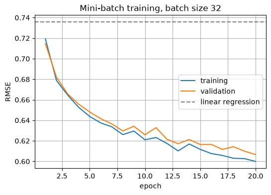
We still want to look at learning curves! We can plot the training and the validation RMSE for each of the epochs to see how we are doing with our learning and look out for overfitting.
After only one epoch the validation RMSE is 0.7146, which already beats linear regression (0.7356). After 20 epochs it is down to 0.6067. The curve drops fast at the start and then slowly. It also wiggles up a little on some epochs (look at epochs 9 and 11), because each step only uses 32 rows, so each step is a little noisy.
NoteQ4. Write this one out by hand
a. There are 15,480 training rows and the batch size is 32. How many steps are in one epoch? How many steps in 20 epochs?
b. Why do we set shuffle=True? What could go wrong if the batches were the same every epoch, or if the rows were sorted by house value?
Comparing the Three Models
# RUN THIS. All three side by side.print("linear regression: ", round(rmse_lin, 4))print("MLP, every row every step, 1000 steps:", round(rmse_mlp, 4))print("MLP, batches of 32, 20 epochs: ", round(valid_rmse[-1], 4))
linear regression:                     0.7356
MLP, every row every step, 1000 steps: 0.602
MLP, batches of 32, 20 epochs:         0.6067
Both MLPs beat linear regression, and they end up close together: 0.602 and 0.6067. What is different is how they got there. Using every row at every step took 1000 passes through the training data. With mini-batches it took 20 passes, and the model had already beaten linear regression after the first one. Each pass with mini-batches makes 484 small updates instead of one, so on a big dataset mini-batches save a lot of time.
NoteQ5. Write this one out by hand
a. Write one sentence about the mini-batch MLP’s validation RMSE in dollars, for somebody who has not taken this class.
b. Look at the learning curve. Are the training and validation RMSE close together or far apart? Is this model overfitting?
Some vocab!
When working with neural networks and MLPs there is lots of vocab you will hear:
Input layer: the features going into the network. It does not compute anything, it just holds the inputs. Our input layer has 8.
Hidden layer and output layer: every layer between the inputs and the output is hidden. The output layer gives the prediction.
Width and depth: the width of a layer is how many neurons it has, and the depth of a network is how many layers it has. Our MLP has one hidden layer of width 50.
Deep Network: a network with many hidden layers. The more hidden layers the deeper the network is.
Wide Network: a network where one or more of the hidden layers has lots of neurons.
Fully connected or dense layer: every input connects to every neuron in the layer. That is what nn.Linear is.
Parameters: the weights and biases the model learns. Our MLP has 501.
Hyperparameters: the choices we make before training, like the number of layers, the width of each layer, the learning rate, the batch size and the number of epochs.
Forward pass and backward pass: the forward pass is running data through the model to get predictions, model(X). The backward pass is computing the gradients, loss.backward().
Feedforward network: the data only moves one way, from the inputs to the output. An MLP is a feedforward network.
Deep learning: machine learning with deep neural networks, meaning many hidden layers.
Putting It Together
Everything from today, in one list:
nn.Linear(inputs, outputs) is a layer of neurons. It holds the weights and biases for you.
An MLP stacks layers with an activation like ReLU between them. Without the activation, the layers collapse into one straight line.
nn.Sequential puts the layers in order.
The loss function (nn.MSELoss for regression) and the optimizer (torch.optim.SGD) replace the lines we wrote by hand last class.
The loop is: zero_grad, predict, loss, backward, step.
Mini-batches use a few rows per step. A DataLoader makes the batches, and one trip through all of them is an epoch.
We will use this same loop for every network we build for the rest of the semester, even when the layers change.
New Commands Today
Command
What it does
The thing that trips people up
.reshape(-1, 1)
turns a list of labels into a column
the model outputs a column, so the labels have to be a column too
nn.Linear(in, out)
a layer of out neurons, each with in inputs
the weights start random, so set torch.manual_seed to get the same numbers twice
nn.ReLU()
the activation \max(0, z)
it goes between layers, not after the last one for regression
nn.Sequential(...)
puts layers in order
the output size of one layer has to match the input size of the next
model.parameters()
every weight and bias in the model
hand it to the optimizer
nn.MSELoss()
mean squared error
take torch.sqrt of it to get the RMSE
torch.optim.SGD(model.parameters(), lr=)
does the update step
lr is the learning rate. Too big and the loss becomes nan
optimizer.zero_grad(), optimizer.step()
clear the gradients, update the weights
forget zero_grad and the gradients add up, like last class
TensorDataset(X, y)
pairs features with labels
X and y need the same number of rows
DataLoader(data, batch_size=, shuffle=True)
cuts the data into batches
one trip through all the batches is one epoch
TipYou Try: optional code
Nothing here is collected. Work through it if you want the idea to stick.
1. Change the hidden layer to 10 neurons, and then to 200. How does the validation RMSE change? How does the training time change?
2. Change the batch size to 256. How many steps are in one epoch now? What happens to the learning curve?
3. Add a second hidden layer: nn.Linear(50, 40) and another nn.ReLU() before the output layer (the output layer becomes nn.Linear(40, 1)). This is the network from the reading.
Before Next Class
In your lecture notes notebook, add your handwritten notes and answers to the questions.
Do the Day 10 practice problems in HW_day10.ipynb. They are practice, not graded, and Weekly Homework 5 assumes you have done them.
Weekly Homework 5 is due Sunday 10/18 at 11:59pm. It covers Day 9 and Day 10.
Day 11 is Tuesday 10/20. Read Geron Appendix A (Autodiff) and chapter 11, the sections Glorot and He Initialization and Better Activation Functions.
Answers to the Q Boxes
Try every one of these by hand first. These are short summaries, not full answers, and the writing out is the part that does the work.
NoteQ1. A layer
a. 50 neurons with 8 weights each is 400 weights, plus 50 biases, so 450 numbers.
b. The sigmoid squashes everything between 0 and 1. A house value of 2.5 ($250,000) would be impossible to predict. For regression the output layer has no activation, so it can give any number.
NoteQ2. The MLP
a. Hidden layer: 8 \times 50 = 400 weights and 50 biases, 450 numbers. Output layer: 50 weights and 1 bias, 51 numbers. 450 + 51 = 501.
b. Without an activation, the two layers are a weighted sum of weighted sums, which is just one weighted sum. The whole model would be one linear regression, like the example in the notes. ReLU turns negative hidden values into 0, which adds a nonlinearity.
NoteQ3. The loop
a.model(X_train_t) is predict, loss_fn(...) is the loss, loss.backward() is backward, optimizer.step() is the update, and optimizer.zero_grad() is the clear. The optimizer’s two lines replaced the update and the clear we wrote by hand.
b. It needs to know which numbers to change and how big a step to take. We gave it both when we made it: model.parameters() and lr. The gradients themselves come from loss.backward(), which stores them in each parameter’s .grad.
NoteQ4. Mini-batches
a.15{,}480 / 32 = 483.75, so 484 steps per epoch (the last batch has 24 rows). 20 epochs is 9,680 steps.
b. If the batches were the same every epoch, the model would see the same groups every time and the steps would repeat the same pattern. If the rows were sorted by house value, one batch would be all cheap houses and the next all expensive ones, and each step would pull the model toward one extreme. Shuffling makes every batch a small random sample of the whole training set.
NoteQ5. The results
a. Something like: “For a neighborhood the model has not seen, its prediction of the median house value is typically off by about $61,000.” (0.6067 times $100,000.)
b. Close together. After 20 epochs the training RMSE is 0.600 and the validation RMSE is 0.6067. The model is not overfitting. Both curves are still going down slowly, so it could train a little longer.