Blue Q boxes are questions for you to answer by hand, in a notebook, with a pen. Not because I am old fashioned. Writing something down by hand is slow, and slow is the point: it is very hard to write an explanation you do not actually understand. You are welcome to use AI in this class for the mechanics of code, but these boxes are the part where you do the thinking yourself. Bring your written notes to class, I will ask to see them.
Green You Try boxes are optional code for you to work through. Nothing is collected and nothing is graded. They are there because you will learn more from changing a number and rerunning than from watching me do it.
Every code cell begins with a tag that tells you what to do with it.
# RUN THIS. Setup, loading data, a plot. Copy it, run it, move on. You do not need to be able to write it from memory.
# LEARN TO WRITE THIS. The pattern of the day. The homework will ask you for it, and so will the exam. Type it out yourself at least once rather than pasting it.
# DEMO ONLY. Code that exists to show one idea. You do not need to be able to write it yourself.
# UNDERSTAND THESE STEPS. Code that shows how something works inside, one small step at a time. Read it and make sure you understand what each line does. You do not need to memorize it or be able to write it from scratch.
Reading: Geron Appendix A (Autodiff), and chapter 11, the sections Glorot and He Initialization and Better Activation Functions.
Last class we built our first neural network, a multilayer perceptron with one hidden layer, and trained it with five lines: zero_grad, predict, loss, backward, step. Today we look inside that loop and ask three questions.
What does loss.backward() actually do? It is called backpropagation, and we will do one by hand on a tiny network to see that it is just the chain rule from calculus.
What happens when we make the network deep? We will stack 10 hidden layers and find out that the network does not learn at all! The reason is in the gradients.
How do we fix it? Two choices decide whether a deep network learns: the activation function and the numbers the weights start at, which is called initialization.
We use the California housing data again, so we can compare to last class. Our one hidden layer MLP got a validation RMSE of 0.6067.
Here is the plan for today:
Do backpropagation by hand on a tiny network.
Build a deep network with the sigmoid activation and watch it fail.
Look at the gradients in each layer to see why.
Try better activation functions.
Look at where the weights start, and learn Kaiming initialization.
Train the deep network.
The California Housing Data, Again
This is the same setup as last class: load the data, split it, scale it with a preprocessing pipeline, and turn it into tensors. The label is the median house value in units of $100,000.
# RUN THIS. Imports, the data, the split, the scaling and the tensors. All of this is from Day 10.import numpy as npimport pandas as pdimport matplotlib.pyplot as pltimport torchimport torch.nn as nnfrom torch.utils.data import TensorDataset, DataLoaderfrom sklearn.model_selection import train_test_splitfrom sklearn.preprocessing import StandardScalerfrom sklearn.pipeline import Pipelinehousing = pd.read_csv("data/california_housing.csv")X = housing.drop(columns=["MedHouseVal"])y = housing["MedHouseVal"]X_train, X_valid, y_train, y_valid = train_test_split( X, y, test_size=0.25, random_state=42)# The preprocessing pipeline, fit on the training rows onlypreprocessing = Pipeline([ ("scale", StandardScaler())])X_train_scaled = preprocessing.fit_transform(X_train)X_valid_scaled = preprocessing.transform(X_valid)# The data as tensors, with the labels as a columnX_train_t = torch.tensor(X_train_scaled, dtype=torch.float32)X_valid_t = torch.tensor(X_valid_scaled, dtype=torch.float32)y_train_t = torch.tensor(y_train.values, dtype=torch.float32).reshape(-1, 1)y_valid_t = torch.tensor(y_valid.values, dtype=torch.float32).reshape(-1, 1)# Pair the features with the labels, so a DataLoader can make batchestrain_data = TensorDataset(X_train_t, y_train_t)print("training rows:", X_train_t.shape)print("validation rows:", X_valid_t.shape)
training rows: torch.Size([15480, 8])
validation rows: torch.Size([5160, 8])
Before we train anything, we want one more number to compare to. What if a model learned nothing at all, and just predicted the average house value for every neighborhood?
# RUN THIS. The RMSE of a model that always predicts the average.mean_value = y_train_t.mean() # the average house value in the training rowserrors = y_valid_t - mean_value # how far off that guess is for every validation rowrmse_mean = torch.sqrt((errors **2).mean()).item() # the RMSE, by handprint("average house value in the training rows:", round(mean_value.item(), 4))print("validation RMSE if we always predict the average:", round(rmse_mean, 4))
average house value in the training rows: 2.0703
validation RMSE if we always predict the average: 1.1503
So a model that knows nothing is typically off by about $115,000. Remember this number, 1.1503. We are going to see it again!
Backpropagation: What Does loss.backward() Do?
We have been calling loss.backward() since Day 9, and it hands us the derivative of the loss with respect to every weight. How does it do that for a whole network?
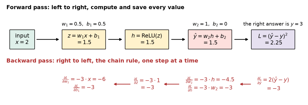
Let’s do it by hand for the smallest network we can build: one input, one hidden neuron with a ReLU, and one output neuron. It has four numbers to learn: w_1, b_1, w_2 and b_2.
We send in one row of data, x = 2, and the right answer is y = 3.
The forward pass
The forward pass is what model(X) does. We go left to right and compute each value from the one before it.
The forward pass for our tiny network. Each box uses the value from the box before it.
The network predicted 1.5 and the right answer is 3, so the loss is (1.5 - 3)^2 = 2.25.
The backward pass
Now we want to know how to change each of the four numbers to make the loss smaller. That means we need four derivatives. The backward pass gets them by starting at the loss and working back toward the input, right to left, using the chain rule from calculus at every step.
The forward pass computes and saves every value. The backward pass starts at the loss and works back, multiplying by one more derivative at each step.
Start at the right. The loss is L = (\hat{y} - y)^2, so
That is all loss.backward() does: the chain rule, one step at a time, starting at the loss and going backward through the network. This is called backpropagation, or backprop for short.
There are two things to notice.
The backward pass reuses values from the forward pass. To get \partial L / \partial w_2 we needed h, and to get through the ReLU we needed to know if z was positive. This is why PyTorch records every calculation when requires_grad=True.
Every step back multiplies by one more number. To get all the way back to w_1 we multiplied three things together. In a network with 10 layers, the gradient for the first layer is a product of many numbers. Remember this for the next section!
NOTE - The reading (Appendix A) calls this reverse-mode autodiff. It is the same idea: go forward once and save the values, then go backward once and get every derivative. One backward pass gives the derivative for every weight in the network, even if there are millions of them.
NoteQ1. Write this one out by hand
a. Redo the forward pass and the backward pass by hand for the same tiny network, but with w_2 = 3 instead of 1. Everything else stays the same. What are the loss and the four derivatives?
b. Why does the backward pass need the values that were saved during the forward pass? Optional Challenge: Do backprop by hand for a slightly more complicated network eg. Logistic regression with one neuron and two input variables.
A Deep Network That Does Not Learn
Last class our MLP had one hidden layer. What if we use 10 hidden layers? More layers means the network can build more complicated patterns out of simpler ones, and that is the “deep” in deep learning. So it should do better… right?
We need two helper functions so that we do not have to retype the same code all day.
The first one builds a network with 10 hidden layers of 50 neurons each. We hand it the activation function we want to use. We do this using a function and a for loop so that we don’t have to type out all the layers!!
# RUN THIS. A function that builds a deep network: 10 hidden layers, 50 neurons each.def make_deep_model(activation): layers = [] # start with an empty list of layers layers.append(nn.Linear(8, 50)) # the first hidden layer: 8 inputs, 50 neurons layers.append(activation()) # the activation that goes after itfor i inrange(9): # 9 more hidden layers, each one 50 neurons wide layers.append(nn.Linear(50, 50)) layers.append(activation()) layers.append(nn.Linear(50, 1)) # the output layer: 1 prediction model = nn.Sequential(*layers) # the * hands the layers in the list to nn.Sequential one at a timereturn modeltorch.manual_seed(42)sigmoid_model = make_deep_model(nn.Sigmoid) # nn.Sigmoid is the sigmoid from Day 9, as a layerprint(sigmoid_model)
The second helper is the mini-batch training loop from last class, inside a function. Nothing in it is new. It returns the validation RMSE after every epoch, so we can plot a learning curve.
If you want to test your understanding of Day10, add comments to the code inside the function. Say in words what each step is doing.
# RUN THIS. The mini-batch training loop from Day 10, inside a function so we can reuse it.def train_model(model, learning_rate, n_epochs): torch.manual_seed(42) # so the batches come in the same order every time train_loader = DataLoader(train_data, batch_size=32, shuffle=True) loss_fn = nn.MSELoss() optimizer = torch.optim.SGD(model.parameters(), lr=learning_rate) valid_rmse = [] for epoch inrange(n_epochs):for X_batch, y_batch in train_loader: optimizer.zero_grad() y_pred = model(X_batch) loss = loss_fn(y_pred, y_batch) loss.backward() optimizer.step()with torch.no_grad(): rmse = torch.sqrt(loss_fn(model(X_valid_t), y_valid_t)).item() valid_rmse.append(rmse)if epoch ==0or (epoch +1) %5==0: # print the first epoch and then every fifth oneprint("epoch", epoch +1, " valid RMSE:", round(rmse, 4))return valid_rmse
Now we train the deep sigmoid network, with the same learning rate and batch size as last class.
# DEMO ONLY. Train the deep network with sigmoid activations.# sigmoid model is the deep neural net we build above# train_model is the function that does the mini-batch training.valid_rmse_sigmoid = train_model(sigmoid_model, learning_rate=0.01, n_epochs=10)
Do you recognize that number? The validation RMSE is stuck at about 1.15, which is what we get by always predicting the average house value (1.1503). After 10 epochs, and 4,840 steps of gradient descent, the network with 10 hidden layers has learned nothing from the features. Our small MLP from last class got 0.6067!
Why? Look at the gradients
Gradient descent changes each weight by the learning rate times its gradient. So if a network is not learning, the first thing to look at is the gradients. Why? Well if the gradients are all zero then the model never takes a step!!!
Lets start with fresh copy of the deep sigmoid network, do one forward pass and one backward pass with all the training rows, and then look at the average size of the gradient in each layer.
# JUST RUN THIS CODE. How big are the gradients in each layer?def print_gradient_sizes(model): loss_fn = nn.MSELoss() loss = loss_fn(model(X_train_t), y_train_t) # forward pass with every training row loss.backward() # backward pass: fills in .grad for every weight layer_number =1for layer in model: # go through the layers in orderifisinstance(layer, nn.Linear): # only the Linear layers have weights grad_size = layer.weight.grad.abs().mean().item() # the average size of the gradients in this layerprint("layer", layer_number, " average gradient size:", round(grad_size, 8)) layer_number = layer_number +1torch.manual_seed(42)sigmoid_model = make_deep_model(nn.Sigmoid) # a fresh copy, not trained yetprint_gradient_sizes(sigmoid_model)
layer 1   average gradient size: 0.0
layer 2   average gradient size: 0.0
layer 3   average gradient size: 3e-08
layer 4   average gradient size: 2.4e-07
layer 5   average gradient size: 1.51e-06
layer 6   average gradient size: 1.094e-05
layer 7   average gradient size: 8.81e-05
layer 8   average gradient size: 0.00062537
layer 9   average gradient size: 0.00544868
layer 10   average gradient size: 0.03911236
layer 11   average gradient size: 2.35417581
Read that list from the bottom up, because that is the direction backprop goes. The last layer (layer 11, the output layer) has a healthy gradient, about 2.35. Every layer we go back, the gradient is roughly ten times smaller. By the time we get to layers 1 and 2 the gradient rounds to 0.
A weight with a gradient of 0 does not change, no matter how many steps we take. So the first layers, the ones that look at the actual features, never learn anything. This is called the vanishing gradients problem.
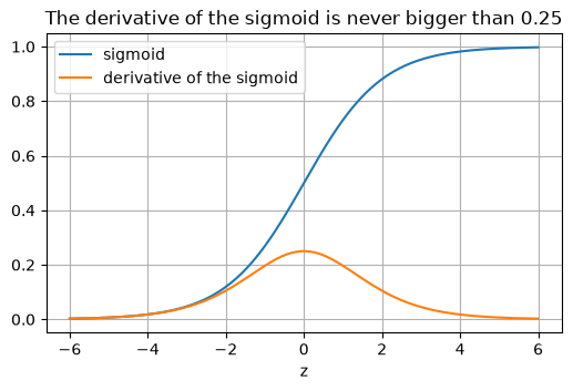
Where does it come from? Remember from the tiny network that every step back multiplies by one more derivative. Going back through a sigmoid means multiplying by the derivative of the sigmoid. Let’s look at it.
# DEMO ONLY. The sigmoid and its derivative.z = torch.linspace(-6, 6, 200)sig = torch.sigmoid(z)sig_derivative = sig * (1- sig) # the derivative of the sigmoid is sigmoid(z) * (1 - sigmoid(z))plt.figure(figsize=(6, 3.5))plt.plot(z, sig, label="sigmoid")plt.plot(z, sig_derivative, label="derivative of the sigmoid")plt.xlabel("z")plt.title("The derivative of the sigmoid is never bigger than 0.25")plt.legend()plt.grid()plt.show()print("biggest value of the derivative:", round(sig_derivative.max().item(), 4))
biggest value of the derivative: 0.2499
The derivative of the sigmoid is at most 0.25, and when z is far from 0 it is almost 0. So every time backprop goes back through a sigmoid layer, the gradient gets multiplied by a number that is 0.25 or smaller. Go back through 10 of them and the gradient vanishes!
This problem stopped people from training deep networks for a long time. The fixes are surprisingly simple, and we will do two of them today.
NoteQ2. Write this one out by hand
a. The derivative of the sigmoid is at most 0.25. Compute 0.25^{3} and 0.25^{10}. What does this tell you about the gradient in the first layer of a network with 3 sigmoid layers compared to one with 10?
Better Activation Functions
The first fix is to stop using the sigmoid between layers.
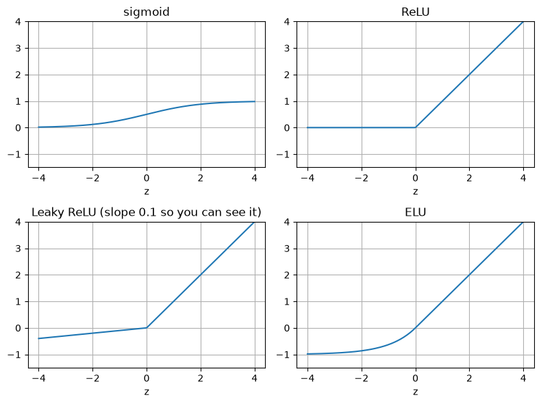
Last class we used ReLU, \text{ReLU}(z) = \max(0, z). Its derivative is exactly 1 for every positive z. Multiplying by 1 does not shrink anything, so the gradient can get back through many layers.
ReLU has one problem of its own. For negative z the output is 0 and the derivative is 0. If a neuron ends up with a negative z for every row of data, it outputs 0 for everything, its gradient is 0, and it can never recover. This is called a dead ReLU. Two popular activations fix this by giving negative numbers a small slope instead of a flat 0:
Leaky ReLU: for negative z it gives 0.01 z, a small slope instead of 0. In PyTorch: nn.LeakyReLU().
ELU (exponential linear unit): for negative z it follows a smooth curve that levels off at -1. In PyTorch: nn.ELU().
Here is what they look like.
# DEMO ONLY. Four activation functions, one plot each.z = torch.linspace(-4, 4, 200)fig, axes = plt.subplots(2, 2, figsize=(8, 6)) # 2 rows and 2 columns of plotsaxes[0, 0].plot(z, torch.sigmoid(z))axes[0, 0].set_title("sigmoid")axes[0, 1].plot(z, torch.relu(z))axes[0, 1].set_title("ReLU")axes[1, 0].plot(z, nn.functional.leaky_relu(z, negative_slope=0.1))axes[1, 0].set_title("Leaky ReLU (slope 0.1 so you can see it)")axes[1, 1].plot(z, nn.functional.elu(z))axes[1, 1].set_title("ELU")for ax in axes.flatten(): # the same settings on all four plots ax.set_xlabel("z") ax.set_ylim(-1.5, 4) ax.grid()plt.tight_layout()plt.show()
The reading talks about more of them (SELU, GELU, Swish). They are all variations on the same idea: do not go flat on both sides the way the sigmoid does. You do not need to memorize them. ReLU is the default choice, and the others are things to try if ReLU is not working.
Let’s swap the sigmoid for ReLU in our deep network. Everything else stays the same. First the gradients:
# DEMO ONLY. The gradient sizes for the same deep network, with ReLU.torch.manual_seed(42)relu_model = make_deep_model(nn.ReLU)print_gradient_sizes(relu_model)
layer 1   average gradient size: 6.9e-06
layer 2   average gradient size: 1.079e-05
layer 3   average gradient size: 1.455e-05
layer 4   average gradient size: 2.041e-05
layer 5   average gradient size: 3.115e-05
layer 6   average gradient size: 0.00012928
layer 7   average gradient size: 0.00032085
layer 8   average gradient size: 0.00084068
layer 9   average gradient size: 0.00278786
layer 10   average gradient size: 0.00756429
layer 11   average gradient size: 0.16840328
The first layer’s gradient is small, about 0.000007, but it is not 0 any more. With the sigmoid the first two layers rounded to 0. Is that enough to learn? Let’s train it.
# DEMO ONLY. Train the deep network with ReLU activations.torch.manual_seed(42)relu_model = make_deep_model(nn.ReLU) # a fresh copy to trainvalid_rmse_relu = train_model(relu_model, learning_rate=0.01, n_epochs=20)
It learns! After 20 epochs the validation RMSE is 0.5754, which beats our one hidden layer MLP from last class (0.6067).
But look at the first few epochs. At epoch 1 and epoch 5 it is still sitting at 1.15, the “predict the average” number. For the first several epochs the deep ReLU network was learning nothing, and then it finally started to learn. Why the slow start? We come back to this in the next section.
First, does ELU do any better?
# DEMO ONLY. The same deep network with ELU activations.torch.manual_seed(42)elu_model = make_deep_model(nn.ELU)valid_rmse_elu = train_model(elu_model, learning_rate=0.01, n_epochs=20)
ELU started learning right away, 0.7373 after the first epoch, but after 20 epochs it ended at 0.5988, a little behind ReLU’s 0.5754. So there is no clear winner here. The big difference is between the sigmoid and everything else:
activation
validation RMSE after 20 epochs
what happened
sigmoid
1.15 (after 10 epochs)
never learned
ReLU
0.5754
stuck for the first several epochs, then learned
ELU
0.5988
learned from the first epoch
NoteQ3. Write this one out by hand
a. What is the derivative of ReLU when z is positive? When z is negative? Why does that help the gradient get back to the first layer, compared to the sigmoid?
b. What is a dead ReLU neuron? How does Leaky ReLU keep that from happening?
Where Should the Weights Start? Initialization
The deep ReLU network sat at 1.15 for the first several epochs before it started to learn. The activation function is fine now, so what was holding it back?
Gradient descent has to start somewhere. The numbers the weights start at are called the initialization, and they matter much more than you would think.
How big is the signal?
Think about the forward pass. The features go into layer 1, the outputs of layer 1 go into layer 2, and so on through all 10 hidden layers. We will call the numbers flowing through the network the signal. If every layer makes the signal a little smaller, then after 10 layers there is almost nothing left.
Let’s measure it. Below we send 1000 training rows through a fresh deep ReLU network, and after each ReLU we print the standard deviation of the numbers coming out. The standard deviation tells us how spread out the signal is. (Our scaled features start with a standard deviation of about 1.)
# DEMO ONLY. How big is the signal after each hidden layer?def print_signal_sizes(model): signal = X_train_t[:1000] # the first 1000 training rows layer_number =1with torch.no_grad(): # we are only looking, not trainingfor layer in model: # send the rows through one layer at a time signal = layer(signal)ifisinstance(layer, nn.ReLU): # after each activation, print how spread out the numbers areprint("after hidden layer", layer_number, " standard deviation:", round(signal.std().item(), 5)) layer_number = layer_number +1torch.manual_seed(42)relu_model = make_deep_model(nn.ReLU) # a fresh copy with PyTorch's default starting weightsprint_signal_sizes(relu_model)
after hidden layer 1   standard deviation: 0.33412
after hidden layer 2   standard deviation: 0.14069
after hidden layer 3   standard deviation: 0.08206
after hidden layer 4   standard deviation: 0.06186
after hidden layer 5   standard deviation: 0.05536
after hidden layer 6   standard deviation: 0.0484
after hidden layer 7   standard deviation: 0.04948
after hidden layer 8   standard deviation: 0.06046
after hidden layer 9   standard deviation: 0.06015
after hidden layer 10   standard deviation: 0.05001
The signal starts at about 0.33 after the first hidden layer and shrinks to about 0.05 by the end. The network is squashing all of its inputs toward 0, so every neighborhood looks almost the same by the time it reaches the output layer. The gradients have the same problem going the other way, which is why they were so small in the first layers.
What decides how big the signal is? The size of the starting weights. Here are two extreme cases, so you can see both ways this can go wrong. nn.init.normal_ fills a layer’s weights with random numbers that have the standard deviation we ask for.
# DEMO ONLY. Starting weights that are too small, and starting weights that are too big.torch.manual_seed(42)small_model = make_deep_model(nn.ReLU)for layer in small_model:ifisinstance(layer, nn.Linear): nn.init.normal_(layer.weight, std=0.01) # tiny random weights. The _ at the end means "change it in place" nn.init.zeros_(layer.bias) # biases start at 0print("TOO SMALL: starting weights with standard deviation 0.01")print_signal_sizes(small_model)print()torch.manual_seed(42)big_model = make_deep_model(nn.ReLU)for layer in big_model:ifisinstance(layer, nn.Linear): nn.init.normal_(layer.weight, std=1.0) # big random weights nn.init.zeros_(layer.bias)print("TOO BIG: starting weights with standard deviation 1")print_signal_sizes(big_model)
TOO SMALL: starting weights with standard deviation 0.01
after hidden layer 1   standard deviation: 0.01577
after hidden layer 2   standard deviation: 0.00094
after hidden layer 3   standard deviation: 5e-05
after hidden layer 4   standard deviation: 0.0
after hidden layer 5   standard deviation: 0.0
after hidden layer 6   standard deviation: 0.0
after hidden layer 7   standard deviation: 0.0
after hidden layer 8   standard deviation: 0.0
after hidden layer 9   standard deviation: 0.0
after hidden layer 10   standard deviation: 0.0

TOO BIG: starting weights with standard deviation 1
after hidden layer 1   standard deviation: 1.57743
after hidden layer 2   standard deviation: 9.44084
after hidden layer 3   standard deviation: 47.15448
after hidden layer 4   standard deviation: 213.37262
after hidden layer 5   standard deviation: 846.32587
after hidden layer 6   standard deviation: 3386.2334
after hidden layer 7   standard deviation: 17179.2832
after hidden layer 8   standard deviation: 100526.9375
after hidden layer 9   standard deviation: 497786.875
after hidden layer 10   standard deviation: 2827710.5
With weights that are too small, the signal is gone (0.0) by the fourth hidden layer. This is the vanishing problem again. With weights that are too big, the signal gets about five times bigger at every layer and ends up in the millions. That is called exploding, and it is where a loss of nan comes from.
So the starting weights need to be just the right size: big enough that the signal does not shrink away, and small enough that it does not explode.
Why not start every weight at the same number?
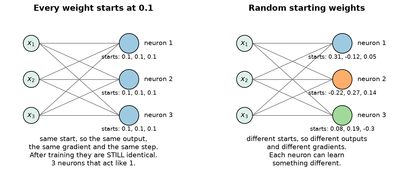
You might wonder why the weights are random at all. On Day 9 we started our one neuron at all zeros and it worked fine. What if we start every weight in a layer at the same number, say 0.1? Here is a picture with 3 hidden neurons.
Left: every weight starts at 0.1, so the neurons stay identical. Right: random starting weights, so each neuron can learn something different.
If all three neurons start the same, they all compute the same output, so they all get the same gradient, so they all take the same step. They will stay identical forever. We paid for 3 neurons and got 1.
Random starting weights break the symmetry: each neuron starts somewhere different, so each one can learn something different. (One neuron on Day 9 had nobody to be the same as, which is why zeros were fine there.)
Xavier and Kaiming initialization
So we want random starting weights that are the right size. How big is right? Two papers worked out the answer. The reading names each method after the first author’s last name, and PyTorch uses the first author’s first name, so each one has two names:
Xavier initialization (the reading calls it Glorot initialization) is for the sigmoid and tanh activations.
Kaiming initialization (the reading calls it He initialization) is for ReLU and its relatives.
We will use the PyTorch names from here on, because those are the names you type in your code.
The idea is the same in both: the more inputs a neuron has, the smaller its weights should be, because it is adding up more things. For Kaiming initialization the weights are random numbers with
\text{standard deviation} = \sqrt{\frac{2}{\text{number of inputs}}}
Our hidden layers have 50 inputs each, so Kaiming initialization uses a standard deviation of \sqrt{2/50} = 0.2. PyTorch’s default starting weights for these layers have a standard deviation of about 0.08. That is on the small side for a deep ReLU network, and that is why our signal was shrinking.
Here is how to ask for Kaiming initialization. We go through the layers of the model, and for every nn.Linear layer we replace its starting weights with nn.init.kaiming_normal_.
# DEMO ONLY. Kaiming initialization for every Linear layer in a model.torch.manual_seed(42)kaiming_model = make_deep_model(nn.ReLU)# Update the initializationsfor layer in kaiming_model: # go through the layers in orderifisinstance(layer, nn.Linear): # only the Linear layers have weights nn.init.kaiming_normal_( layer.weight, # the weights to fill in nonlinearity="relu") # which activation comes after this layer nn.init.zeros_(layer.bias) # start the biases at 0print_signal_sizes(kaiming_model)
after hidden layer 1   standard deviation: 0.78872
after hidden layer 2   standard deviation: 0.94408
after hidden layer 3   standard deviation: 0.94309
after hidden layer 4   standard deviation: 0.85349
after hidden layer 5   standard deviation: 0.67706
after hidden layer 6   standard deviation: 0.5418
after hidden layer 7   standard deviation: 0.54974
after hidden layer 8   standard deviation: 0.64337
after hidden layer 9   standard deviation: 0.63717
after hidden layer 10   standard deviation: 0.72389
Now the signal stays between about 0.5 and 0.9 all the way through the 10 hidden layers. It does not shrink away and it does not explode. A healthy signal going forward also means healthy gradients going backward, so now the first layers get a gradient they can learn from.
NoteQ4. Write this one out by hand
a. Why can we not start every weight in a layer at the same number? What happens to the 3 hidden neurons in the picture?
b. A hidden layer has 200 inputs. What standard deviation does Kaiming initialization use for its weights? What goes wrong in a deep network if the starting weights are much smaller than that? What if they are much bigger?
Training the Deep Network
Now we train the deep ReLU network with Kaiming initialization.
BEWARE! If we use the learning rate from before, 0.01, the loss is nan. We saw this last class: the steps were too big. Each step is the learning rate times the gradient, and Kaiming initialization made the gradients much bigger, so the same learning rate now takes much bigger steps. Remember: if you ever see nan in your loss, the first thing to try is a smaller learning rate. So we use 0.001.
# DEMO ONLY. Build the model, set the starting weights, then train.torch.manual_seed(42)kaiming_model = make_deep_model(nn.ReLU)# Update the initializationsfor layer in kaiming_model:ifisinstance(layer, nn.Linear): nn.init.kaiming_normal_(layer.weight, nonlinearity="relu") nn.init.zeros_(layer.bias)valid_rmse_kaiming = train_model(kaiming_model, learning_rate=0.001, n_epochs=20)
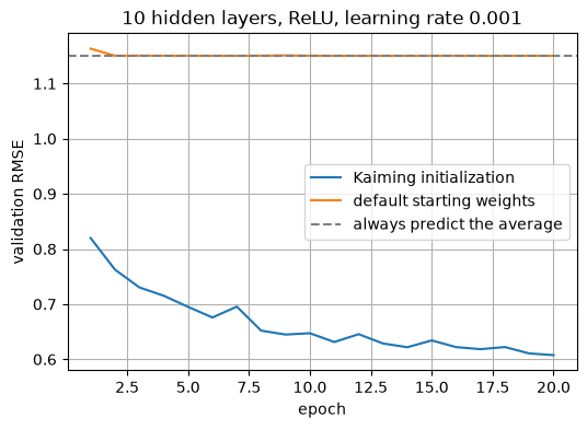
It learns from the very first epoch: 0.8198 after one epoch, and 0.6076 after 20.
To be fair we should compare to the default starting weights at the same learning rate. The only thing that is different between these two runs is where the weights start.
# DEMO ONLY. The same network and the same learning rate, with PyTorch's default starting weights.torch.manual_seed(42)default_model = make_deep_model(nn.ReLU)valid_rmse_default = train_model(default_model, learning_rate=0.001, n_epochs=20)
# RUN THIS. The two learning curves.epochs =range(1, 21)plt.figure(figsize=(6, 4))plt.plot(epochs, valid_rmse_kaiming, label="Kaiming initialization")plt.plot(epochs, valid_rmse_default, label="default starting weights")plt.axhline(rmse_mean, color="gray", linestyle="--", label="always predict the average")plt.xlabel("epoch")plt.ylabel("validation RMSE")plt.title("10 hidden layers, ReLU, learning rate 0.001")plt.legend()plt.grid()plt.show()
With the default starting weights the network sits on the dashed line for all 20 epochs. It never starts to learn. With Kaiming initialization it starts learning right away.
Here is everything we tried today with the 10 hidden layer network:
activation
starting weights
learning rate
validation RMSE after 20 epochs
sigmoid
default
0.01
1.15, never learned (we stopped at 10 epochs)
ReLU
default
0.01
0.5754, stuck for the first several epochs
ELU
default
0.01
0.5988
ReLU
Kaiming
0.001
0.6076, learned from the first epoch
The big lesson is the first row: with the sigmoid, a deep network does not learn at all. ReLU, ELU and Kaiming initialization all fix that. The activation, the starting weights and the learning rate all affect each other, so you try things and look at the learning curve. On Thursday we get tools that let us take big steps and keep training stable: better optimizers, learning rate schedules and batch normalization.
NoteQ5. Write this one out by hand
a. With Kaiming initialization, a learning rate of 0.01 gave nan but 0.001 worked. With the default starting weights, 0.01 worked. Explain why the starting weights change which learning rate works.
b. Look at the learning curve plot. Describe each curve in one sentence. If you could only train for 3 epochs, which starting weights would you use?
Putting It Together
What this looks like in real life
All day we used helper functions like make_deep_model and train_model so we could run the same experiment over and over. In a real project you do not need any of that, although you are welcome to write helper functions and it is a good thing to practice. Here is the whole process in one cell, with comments that show the places you could change things.
# LEARN TO WRITE THIS. # A deep network from start to finish, the way you would write it for a real project.torch.manual_seed(42)# 1. The model. Here you could change the number of layers, the number of neurons,# or the activation, eg. nn.ELU() or nn.LeakyReLU() instead of nn.ReLU()model = nn.Sequential( nn.Linear(8, 50), # 8 features in, 50 neurons nn.ReLU(), nn.Linear(50, 50), nn.ReLU(), nn.Linear(50, 50), nn.ReLU(), nn.Linear(50, 1)) # 1 prediction out# 2. The starting weights. Here you could change the initialization,# or delete this loop to use PyTorch's default starting weightsfor layer in model:ifisinstance(layer, nn.Linear): # only the Linear layers have weights nn.init.kaiming_normal_(layer.weight, nonlinearity="relu") nn.init.zeros_(layer.bias)# 3. The batches, the loss and the optimizer. Here you could change the batch size or the learning ratetrain_loader = DataLoader(train_data, batch_size=32, shuffle=True)loss_fn = nn.MSELoss()optimizer = torch.optim.SGD(model.parameters(), lr=0.001)# 4. The training loop from Day 10n_epochs =20for epoch inrange(n_epochs):for X_batch, y_batch in train_loader: optimizer.zero_grad() # clear the old gradients y_pred = model(X_batch) # forward pass loss = loss_fn(y_pred, y_batch) # how far off are we? loss.backward() # backward pass, this is backpropagation optimizer.step() # one step of gradient descent# 5. Every 5 epochs, check the validation RMSEif (epoch +1) %5==0:with torch.no_grad(): rmse = torch.sqrt(loss_fn(model(X_valid_t), y_valid_t)).item()print("epoch", epoch +1, " valid RMSE:", round(rmse, 4))
Backpropagation is what loss.backward() does. It is the chain rule, starting at the loss and going backward one layer at a time, reusing the values saved in the forward pass.
Every step back multiplies the gradient by one more number. In a deep network those products can get tiny (vanishing gradients) or huge (exploding gradients).
The sigmoid makes gradients vanish, because its derivative is never bigger than 0.25. Use ReLU between layers. Leaky ReLU and ELU are relatives that do not go flat for negative numbers.
Weights have to start random, or every neuron in a layer learns the same thing.
They also have to start at the right size. Kaiming initialization is the standard choice for ReLU: nn.init.kaiming_normal_.
The activation, the starting weights and the learning rate all affect each other. If the loss is nan, try a smaller learning rate first.
New Commands Today
Command
What it does
The thing that trips people up
nn.Sigmoid(), nn.LeakyReLU(), nn.ELU()
activation functions, used as layers in nn.Sequential
they go between layers, just like nn.ReLU()
for layer in model:
goes through the layers of an nn.Sequential in order
the activations are layers too, so check which kind you have
isinstance(layer, nn.Linear)
True if this layer is an nn.Linear
only the Linear layers have .weight and .bias
layer.weight, layer.bias
the weights and biases of one layer
after loss.backward(), the gradients are in layer.weight.grad
the _ at the end means it changes the weights in place. Do it before training
nn.init.zeros_(layer.bias)
sets the biases to 0
fine for biases, never for the weights
nn.init.normal_(layer.weight, std=)
random weights with the standard deviation you ask for
too small and the signal vanishes, too big and it explodes
tensor.std()
the standard deviation of the numbers in a tensor
add .item() to get a plain number
TipYou Try: optional code
Nothing here is collected. Work through it if you want the idea to stick.
1. Train the deep network with nn.LeakyReLU and the default starting weights, with a learning rate of 0.01 for 20 epochs. Is it any different from ReLU?
2. Xavier initialization (Glorot in the reading) is the one to use with the sigmoid. Try it on the deep sigmoid network: replace nn.init.kaiming_normal_(layer.weight, nonlinearity="relu") with nn.init.xavier_uniform_(layer.weight). Print the gradient sizes. Does the deep sigmoid network learn now?
Before Next Class
In your lecture notes notebook, add your handwritten notes and answers to the questions.
Do the Day 11 practice problems in HW_day11.ipynb. They are practice, not graded, and Weekly Homework 6 assumes you have done them.
Weekly Homework 6 is due Sunday 11/1 at 11:59pm (moved: Thursday 10/22 is a Catch-Up Day). It covers Day 11 and Day 12.
Final project: more about the teams and the proposal soon.
Read Geron chapter 11, the sections Batch Normalization, Faster Optimizers and Learning Rate Scheduling.
Answers to the Q Boxes
Try every one of these by hand first. These are short summaries, not full answers, and the writing out is the part that does the work.
NoteQ1. Backpropagation
a. Forward: z = 1.5, h = 1.5, \hat{y} = 3 \cdot 1.5 + 0 = 4.5, and the loss is (4.5 - 3)^2 = 2.25. Backward: \partial L / \partial \hat{y} = 2(4.5 - 3) = 3. Then \partial L / \partial w_2 = 3 \cdot 1.5 = 4.5, \partial L / \partial b_2 = 3 and \partial L / \partial h = 3 \cdot 3 = 9. Through the ReLU, \partial L / \partial z = 9. Last, \partial L / \partial w_1 = 9 \cdot 2 = 18 and \partial L / \partial b_1 = 9. The loss is the same as before, but now the prediction is too big, so the derivatives are positive.
b. Each step back multiplies by a derivative that depends on a value from the forward pass. For example \partial L / \partial w_2 = \partial L / \partial \hat{y} \cdot h needs h, and going back through the ReLU needs to know whether z was positive or negative.
NoteQ2. Vanishing gradients
a.0.25^3 \approx 0.016 and 0.25^{10} \approx 0.00000095. With 3 sigmoid layers the first layer’s gradient is shrunk by a factor of about 60 at worst, which is small but still usable. With 10 layers it is shrunk by about a million, so the first layers barely change.
NoteQ3. Activations
a. 1 when z is positive, 0 when z is negative. Going back through a ReLU with a positive z multiplies the gradient by 1, so it does not shrink. Going back through a sigmoid multiplies it by 0.25 or less every time.
b. A neuron whose z is negative for every row. It outputs 0, its gradient is 0, so its weights never change and it stays that way. Leaky ReLU has a small slope (0.01) for negative z, so the gradient is small but not 0 and the neuron can recover.
NoteQ4. Initialization
a. If every weight in a layer starts the same, every neuron in that layer computes the same output and gets the same gradient, so they all take the same step and stay identical. In the picture the 3 hidden neurons start the same, so they stay identical and act like 1 neuron.
b.\sqrt{2/200} = 0.1. Much smaller: the signal shrinks at every layer and so do the gradients, so the first layers do not learn (vanishing). Much bigger: the signal and the gradients grow at every layer (exploding) and the loss becomes nan.
NoteQ5. Training
a. Each step is the learning rate times the gradient. Kaiming initialization made the gradients much bigger, so a learning rate of 0.01 took steps that were too big and the loss became nan. With the small default gradients, 0.01 was fine, and 0.001 was too small to get anywhere in 20 epochs.
b. Kaiming initialization: the RMSE drops from the first epoch and keeps going down, to 0.6076. Default starting weights: flat on the dashed line at 1.15 for all 20 epochs, it never learns. With only 3 epochs, Kaiming initialization.