Blue Q boxes are questions for you to answer by hand, in a notebook, with a pen. Not because I am old fashioned. Writing something down by hand is slow, and slow is the point: it is very hard to write an explanation you do not actually understand. You are welcome to use AI in this class for the mechanics of code, but these boxes are the part where you do the thinking yourself. Bring your written notes to class, I will ask to see them.
Green You Try boxes are optional code for you to work through. Nothing is collected and nothing is graded. They are there because you will learn more from changing a number and rerunning than from watching me do it.
Every code cell begins with a tag that tells you what to do with it.
# RUN THIS. Setup, loading data, a plot. Copy it, run it, move on. You do not need to be able to write it from memory.
# LEARN TO WRITE THIS. The pattern of the day. The homework will ask you for it, and so will the exam. Type it out yourself at least once rather than pasting it.
# DEMO ONLY. Code that exists to show one idea. You do not need to be able to write it yourself.
# UNDERSTAND THESE STEPS. Code that shows how something works inside, one small step at a time. Read it and make sure you understand what each line does. You do not need to memorize it or be able to write it from scratch.
Reading: Geron chapter 11, the sections Batch Normalization, Faster Optimizers and Learning Rate Scheduling.
Last class we got a network with 10 hidden layers to learn. It needed the ReLU activation and Kaiming initialization, and then it learned from the very first epoch. But there was a problem: we had to turn the learning rate down to 0.001 to keep the loss from becoming nan, and with steps that small the network only got to a validation RMSE of 0.6076 after 20 epochs. Our one hidden layer MLP from Day 10 got 0.6067!
So the deep network learns, but slowly. Today we look at three tools for training faster. None of them change the network’s layers or the data. They change how we take the steps.
Better optimizers. So far every step has been plain gradient descent, torch.optim.SGD. We will add momentum, and then use Adam, which is the optimizer most people reach for first.
Learning rate schedules. Instead of one learning rate for the whole training run, we start with bigger steps and make them smaller as we go.
Batch normalization. A new kind of layer that keeps the signal a good size during training, not just at the start.
We keep the same California housing data and the same network with 10 hidden layers, so every number today can be compared to last class.
The Setup from Last Class - Same Data, Same Deep Network
The first cell is the same data setup as Day 10 and Day 11.
# RUN THIS. Imports, the data, the split, the scaling and the tensors. All of this is from Day 10.import numpy as npimport pandas as pdimport matplotlib.pyplot as pltimport torchimport torch.nn as nnfrom torch.utils.data import TensorDataset, DataLoaderfrom sklearn.model_selection import train_test_splitfrom sklearn.preprocessing import StandardScalerfrom sklearn.pipeline import Pipelinehousing = pd.read_csv("data/california_housing.csv")X = housing.drop(columns=["MedHouseVal"])y = housing["MedHouseVal"]X_train, X_valid, y_train, y_valid = train_test_split( X, y, test_size=0.25, random_state=42)# The preprocessing pipeline, fit on the training rows onlypreprocessing = Pipeline([ ("scale", StandardScaler())])X_train_scaled = preprocessing.fit_transform(X_train)X_valid_scaled = preprocessing.transform(X_valid)# The data as tensors, with the labels as a columnX_train_t = torch.tensor(X_train_scaled, dtype=torch.float32)X_valid_t = torch.tensor(X_valid_scaled, dtype=torch.float32)y_train_t = torch.tensor(y_train.values, dtype=torch.float32).reshape(-1, 1)y_valid_t = torch.tensor(y_valid.values, dtype=torch.float32).reshape(-1, 1)# Pair the features with the labels, so a DataLoader can make batchestrain_data = TensorDataset(X_train_t, y_train_t)print("training rows:", X_train_t.shape)print("validation rows:", X_valid_t.shape)
training rows: torch.Size([15480, 8])
validation rows: torch.Size([5160, 8])
Next are the helper functions. The first two are from last class: one builds the network with 10 hidden layers of 50 neurons and ReLU, and one does Kaiming initialization (it is the loop we wrote last class, inside a function). We use these so we can run the same experiment over and over. At the end of today there is a “real life” cell with no helper functions.
# RUN THIS. The deep network and Kaiming initialization from Day 11.def make_deep_model(): layers = [] # start with an empty list of layers layers.append(nn.Linear(8, 50)) # the first hidden layer: 8 inputs, 50 neurons layers.append(nn.ReLU())for i inrange(9): # 9 more hidden layers, each one 50 neurons wide layers.append(nn.Linear(50, 50)) layers.append(nn.ReLU()) layers.append(nn.Linear(50, 1)) # the output layer: 1 prediction model = nn.Sequential(*layers) # the * hands the layers in the list to nn.Sequential one at a timereturn modeldef kaiming_initialize(model):for layer in model: # go through the layers in orderifisinstance(layer, nn.Linear): # only the Linear layers have weights nn.init.kaiming_normal_(layer.weight, nonlinearity="relu") nn.init.zeros_(layer.bias)
The training function has one important change from last class. Before, it made the optimizer itself, and it was always torch.optim.SGD. Today the optimizer is the thing we are experimenting with, so now the optimizer is an imput to the function so we can play around with it.
There are also three new lines, marked NEW. model.train() and model.eval() are for batch normalization at the end of today, and the scheduler lines are for learning rate schedules. We explain them when we get there!! Look through this code for familiar things! There is a lot here that we have seen before.
# RUN THIS. The mini-batch training loop. The optimizer is now something we hand in.def train_model(model, optimizer, n_epochs, scheduler=None): torch.manual_seed(42) # so the batches come in the same order every time train_loader = DataLoader(train_data, batch_size=32, shuffle=True) loss_fn = nn.MSELoss() valid_rmse = [] # save the validation RMSE after every epochfor epoch inrange(n_epochs): model.train() # NEW: tell the model we are trainingfor X_batch, y_batch in train_loader: # the same five steps as always optimizer.zero_grad() y_pred = model(X_batch) loss = loss_fn(y_pred, y_batch) loss.backward() optimizer.step() model.eval() # NEW: tell the model we are only predicting nowwith torch.no_grad(): rmse = torch.sqrt(loss_fn(model(X_valid_t), y_valid_t)).item() valid_rmse.append(rmse)if scheduler isnotNone: # NEW: if we were given a schedule, tell it an epoch is done scheduler.step()if epoch ==0or (epoch +1) %5==0: # print the first epoch and then every fifth oneprint("epoch", epoch +1, " valid RMSE:", round(rmse, 4))return valid_rmse
Where we left off - The Number to Beat
Here is last class’s best run again, so we have a learning curve to compare to: Kaiming initialization, plain SGD, learning rate 0.001.
# LEARN TO WRITE THIS. Build the model, set the starting weights, make the optimizer, train.torch.manual_seed(42)sgd_model = make_deep_model()kaiming_initialize(sgd_model)sgd_optimizer = torch.optim.SGD( sgd_model.parameters(), # the numbers the optimizer is allowed to change lr=0.001) # the learning ratevalid_rmse_sgd = train_model(sgd_model, sgd_optimizer, n_epochs=20)
Plain gradient descent only looks at the gradient right now. Every step is
w = w - \eta \cdot \text{gradient}
and then it forgets everything. If the gradient is small, the step is small, even if the last hundred gradients all pointed the same way.
Momentum remembers how the gradient was over the past steps. It keeps a running total of the recent gradients, called the velocity, and steps using the velocity instead of the gradient:
v = \beta \cdot v + \text{gradient} \qquad\qquad w = w - \eta \cdot v
The number \beta (beta) is the momentum, and it is almost always 0.9. Each step keeps 90 percent of the old velocity and adds the new gradient on top.
So, what does that do? Pretend the gradient is exactly 1 at every step. With plain gradient descent every step has a size of 1 (times the learning rate). With momentum the velocity keeps building: 1, then 0.9 \cdot 1 + 1 = 1.9, then 0.9 \cdot 1.9 + 1 = 2.71, and it levels off at about 10. So when the gradients keep pointing the same way, momentum takes steps that are up to ten times bigger with the same learning rate. If we are consistently moving in the same direction why not take bigger steps!
And when the gradients keep changing sign, bouncing back and forth, they cancel each other out inside the velocity. So momentum also smooths out the noise we get from using small batches and taking steps in different directioins.
In PyTorch momentum is implemented by adding just one extra argument to torch.optim.SGD.
# LEARN TO WRITE THIS. SGD with momentum.torch.manual_seed(42)momentum_model = make_deep_model()kaiming_initialize(momentum_model)momentum_optimizer = torch.optim.SGD( momentum_model.parameters(), lr=0.001, # the same learning rate as before momentum=0.9) # THE ONLY CHANGE! keep 90 percent of the old velocity at every step valid_rmse_momentum = train_model(momentum_model, momentum_optimizer, n_epochs=20)
This is the same network, same starting weights, and same learning rate. The only thing we changed is momentum=0.9, and the validation RMSE after 20 epochs went from 0.6076 to 0.5454.
NoteQ1. Write this one out by hand
a. Use v = 0.9 \cdot v + \text{gradient}, starting from v = 0. The gradients for the first four steps are 1, 1, -1, -1. Compute the velocity after each step. What happened when the gradient changed sign?
b. In your own words, why does momentum speed up training when the gradients keep pointing the same way?
Adam - A Step Size for Every Weight
Momentum helped a lot! But there is another problem with plain gradient descent: every weight uses the same learning rate.
Remember the gradient sizes from last class. In the same network, some layers had gradients thousands of times bigger than others. So how do we pick one learning rate that works for all of them?
Adam (adaptive moment estimation) gives every weight its own step size. It needs two things to do this:
It keeps a velocity for each weight, like momentum.
It keeps track of how big each weight’s gradients have been lately, and divides the step by that size. A weight whose gradients have been huge gets its steps scaled down. A weight whose gradients have been tiny gets its steps scaled up.
That second idea is what “adaptive” means: the step size adapts to each weight. (The reading calls the second idea by itself RMSProp. Adam is momentum plus RMSProp.)
In PyTorch it is one line, and the rest of the loop stays exactly the same. A learning rate of 0.001 is the usual place to start with Adam.
# LEARN TO WRITE THIS. The Adam optimizer.torch.manual_seed(42)adam_model = make_deep_model()kaiming_initialize(adam_model)adam_optimizer = torch.optim.Adam( adam_model.parameters(), lr=0.001) # 0.001 is the usual starting point for Adamvalid_rmse_adam = train_model(adam_model, adam_optimizer, n_epochs=20)
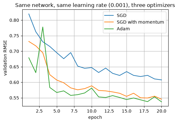
Wow! After just one epoch Adam is at 0.6788, and after 20 epochs it is at 0.537. That is the best we have seen so far on this data!
Let’s put all three optimizers on one plot so we can compare them.
# RUN THIS. The three learning curves.epochs =range(1, 21)plt.figure(figsize=(6, 4))plt.plot(epochs, valid_rmse_sgd, label="SGD")plt.plot(epochs, valid_rmse_momentum, label="SGD with momentum")plt.plot(epochs, valid_rmse_adam, label="Adam")plt.xlabel("epoch")plt.ylabel("validation RMSE")plt.title("Same network, same learning rate (0.001), three optimizers")plt.legend()plt.grid()plt.show()
Both momentum and Adam are well below plain SGD. Notice also that the momentum and Adam curves are bumpier. Look at Adam at epoch 3. Bigger steps get us down faster, but sometimes they step too far and the validation RMSE goes back up for a bit.
NoteQ2. Write this one out by hand
a. In your own words, what does “adaptive” mean in the name Adam? What two things does Adam keep track of for each weight?
b. Look at the plot of the three optimizers. Why are the momentum and Adam curves bumpier than plain SGD?
Learning Rate Schedules - Big Steps First, Small Steps Later
So far we have used one learning rate for the whole training run. But what do we actually want from our learning rate?
Early in training we are far from a good answer. We want big steps so we get there quickly.
Late in training we are close. Big steps now jump around the good answer instead of landing on it. We want small steps.
We can’t get both of these with one learning rate. So why not change the learning rate as we go? A learning rate schedule does exactly that. We start with a big learning rate and make it smaller as we train.
The simplest one is StepLR. It multiplies the learning rate by a number (gamma) every so many epochs (step_size). With step_size=10 and gamma=0.1, starting from 0.001, the learning rate does this:
epochs
learning rate
1 to 10
0.001
11 to 20
0.0001
21 to 30
0.00001
To use a schedule in real training there are two things to do:
Make a scheduler object and hand it the optimizer. This should be done after initializing the optimizer!
Call scheduler.step()once per epoch, after that epoch’s batches are done. We added this as an extra line in the train_model function above.
BEWARE! optimizer.step() and scheduler.step() are different things. optimizer.step() updates the weights and happens once per batch. This is how we LEARN the weights. scheduler.step() updates the learning rate and happens once per epoch. This is how we change the learning rate to get smaller as we get closer to the right answer.
# LEARN TO WRITE THIS. Adam with a learning rate schedule.torch.manual_seed(42)schedule_model = make_deep_model()kaiming_initialize(schedule_model)schedule_optimizer = torch.optim.Adam(schedule_model.parameters(), lr=0.001)scheduler = torch.optim.lr_scheduler.StepLR( schedule_optimizer, # the scheduler changes the learning rate inside this optimizer step_size=10, # every 10 epochs... gamma=0.1) # ...multiply the learning rate by 0.1valid_rmse_schedule = train_model(schedule_model, schedule_optimizer, n_epochs=20, scheduler=scheduler)
# RUN THIS. Adam with and without the schedule.plt.figure(figsize=(6, 4))plt.plot(epochs, valid_rmse_adam, label="Adam, learning rate 0.001 the whole time")plt.plot(epochs, valid_rmse_schedule, label="Adam, learning rate drops to 0.0001 after epoch 10")plt.axvline(10.5, color="gray", linestyle="--")plt.xlabel("epoch")plt.ylabel("validation RMSE")plt.title("Adam with and without a learning rate schedule")plt.legend()plt.grid()plt.show()print("last five epochs without the schedule:", np.round(valid_rmse_adam[15:], 4))print("last five epochs with the schedule: ", np.round(valid_rmse_schedule[15:], 4))
last five epochs without the schedule: [0.5492 0.5434 0.5375 0.5531 0.537 ]
last five epochs with the schedule:    [0.5361 0.5365 0.5348 0.5354 0.5336]
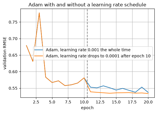
For the first 10 epochs the two curves are exactly the same, because the learning rate is the same. After the dashed line the schedule drops the learning rate to 0.0001.
Look at the last five epochs. Without the schedule the validation RMSE keeps bouncing around (blue line): 0.5492, 0.5434, 0.5375, 0.5531, 0.537. With the schedule it barely moves (orange line): 0.5361, 0.5365, 0.5348, 0.5354, 0.5336.
The final number is only a little better, 0.5336 vs 0.537. So was it worth it? Yes! With the schedule the model is steady at the end. Without the schedule, how good our model is depends on which epoch we happened to stop on.
NOTE - StepLR is the simplest schedule. The reading describes several more, and PyTorch has them all in torch.optim.lr_scheduler. For example ExponentialLR multiplies the learning rate by gamma every single epoch, and ReduceLROnPlateau watches the validation score and lowers the learning rate when it stops improving. They all lower the learning rate as training goes on just using different schedules.
NoteQ3. Write this one out by hand
a. A StepLR schedule has step_size=5 and gamma=0.5, and the optimizer starts with a learning rate of 0.01. What is the learning rate during epoch 3? Epoch 8? Epoch 13?
b. Why do we want big steps early in training and small steps late in training?
Batch Normalization - Keeping the Signal a Good Size During Training
Last class we cared a lot about the size of the signal going through the network. Kaiming initialization made the signal a good size at the start. But as soon as training begins the weights change as we learn, and there is no guarantee that the signal stays a good size.
Batch normalization is a layer that we can add to the sequential network just before the activation function. It keeps the signal a good size during training. It sounds complicated, but it is just StandardScaler on the values of each neuron in the layer. This is happening inside the network.
A batch normalization layer does this for every neuron in the layer:
Take that neuron’s outputs for all the rows in the current batch, x_i.
Subtract their mean and divide by their standard deviation (StandardScaler), \hat{x}_i = \frac{x_i - \mu}{\sigma}. Now the outputs have mean 0 and standard deviation 1.
Multiply by a scale and add a shift to allow the model to learn the best choice for mean and standard deviation.
Now step three might be a bit confusing… but basicaly we take each neurons output that has been put through a StandardScaler, \hat{x}_i, and then give the model some flexibility to decide if we really should have used a mean of zero and a standard deviation of one. We do this by shifting and squeezing the function:
z_i = \gamma \hat{x}_i + \beta
This gives us TWO MORE PARAMETERS for every neuron that we need to learn during gradient decent. This value z_i is what is sent through the activation funciton and on forward through the network.
In PyTorch it is nn.BatchNorm1d, and it goes between the nn.Linear layer and the activation. The number you give it is how many neurons are in the layer before it.
# LEARN TO WRITE THIS. A small network with a batch normalization layer.torch.manual_seed(42)small_bn_model = nn.Sequential( nn.Linear(8, 50), nn.BatchNorm1d(50), # standardize the 50 outputs of the layer above, using the current batch nn.ReLU(), nn.Linear(50, 1))print(small_bn_model)# How many numbers does the batch normalization layer learn?bn_layer = small_bn_model[1] # layer number 1 is the BatchNorm1d (we start counting at 0)print()print("scale, one per neuron:", bn_layer.weight.shape)print("shift, one per neuron:", bn_layer.bias.shape)
Sequential(
  (0): Linear(in_features=8, out_features=50, bias=True)
  (1): BatchNorm1d(50, eps=1e-05, momentum=0.1, affine=True, bias=True, track_running_stats=True)
  (2): ReLU()
  (3): Linear(in_features=50, out_features=1, bias=True)
)

scale, one per neuron: torch.Size([50])
shift, one per neuron: torch.Size([50])
The layer learns 50 scales and 50 shifts, 100 numbers in all.
Notice there are lots of default variables int he BatchNorm1d:
Setting
What it means
50
Number of neurons coming in from the layer before. It has to match, eg. nn.Linear(8, 50).
eps=1e-05
A tiny number added inside the square root, \hat{x} = \frac{x-\mu}{\sqrt{\sigma^2 + \epsilon}}, so we never divide by 0 if a neuron’s outputs are all the same in a batch.
momentum=0.1
How fast the running averages (the ones model.eval() uses) update
affine=True
Learn the scale \gamma and shift \beta, linear. With False it only standardizes.
bias=True
Learn the shift \beta. On by default when affine=True.
track_running_stats=True
Keep the running averages during training so model.eval() has something to use. With False it uses the current batch even in prediction mode.
NOTE - The momentum here is NOT the optimizer momentum from earlier today! We will learn more about this next.
Training mode and prediction mode - model.train() and model.eval()
Here is one thing about batch normalization that trips everybody up, so read this part carefully.
While we train, the layer uses the mean and standard deviation of the current batch. That means the prediction for one house depends on which other houses happen to be in the batch with it! That is fine while we are training, but it is a terrible way to make real predictions. The price we predict for a house should not depend on which other houses we looked up that day.
So while it trains, the layer also keeps a running average of the means and standard deviations it has seen. When we switch the model to prediction mode with model.eval(), it stops using the batch data and instead uses those saved averages that it compiled while it was learning.
This explains two more of the new lines in the training loop function above:
model.train() before the training batches - tells the model to calculate the average and standard deviation for each batch and track the running average.
model.eval() before predicting on the validation set - tells the model that we are done training and that we should use the running average during prediction.
BEWARE! If you forget model.eval(), your validation predictions get computed with batch statistics and your scores will be wrong. Nothing will crash and there will be no error message. From now on we put these two lines in every training loop, even when the model has no batch normalization, so that we never forget.
On our small housing network batch normalization does not make a big difference, so we will not train with it today. Where it really matters is in much deeper networks. You will see it again inside the convolutional neural networks (CNNs) we build for images, and a very similar layer called layer normalization is inside every transformer.
NoteQ4. Write this one out by hand
a. In your own words, what does a batch normalization layer do to the outputs of the layer before it? Where does it go in an nn.Sequential?
b. What is different about a batch normalization layer in training mode and in prediction mode? What goes wrong if you forget model.eval() before you predict on the validation set?
Comparing Everything - What Should You Use?
# RUN THIS. Everything from today on one plot.plt.figure(figsize=(7, 4.5))plt.plot(epochs, valid_rmse_sgd, label="SGD, lr 0.001")plt.plot(epochs, valid_rmse_momentum, label="SGD with momentum, lr 0.001")plt.plot(epochs, valid_rmse_adam, label="Adam, lr 0.001")plt.plot(epochs, valid_rmse_schedule, label="Adam with a schedule")plt.xlabel("epoch")plt.ylabel("validation RMSE")plt.title("10 hidden layers, four ways to train")plt.legend()plt.grid()plt.show()
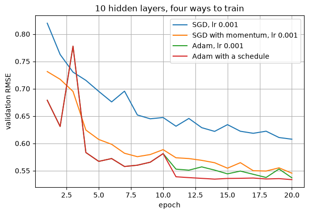
Here is everything we tried today, all with the same network of 10 hidden layers and 20 epochs:
how we trained it
validation RMSE after 20 epochs
SGD, learning rate 0.001 (last class)
0.6076
SGD with momentum 0.9, learning rate 0.001
0.5454
Adam, learning rate 0.001
0.537
Adam with a StepLR schedule
0.5336
Every one of these beat where we started. So what should you actually use? Here is my default recipe for a new problem:
ReLU activations and Kaiming initialization (last class).
Adam with a learning rate of 0.001.
Look at the learning curve. If it is bouncing around at the end, add a schedule.
If a very deep network will not train, or gives nan, try a smaller learning rate first, then batch normalization.
One more thing to notice - A Hint of Overfitting
All day we have only looked at the validation RMSE. Let’s also look at the training RMSE for the Adam model.
# RUN THIS. Training RMSE and validation RMSE for the Adam model.loss_fn = nn.MSELoss()adam_model.eval()with torch.no_grad(): train_rmse_adam = torch.sqrt(loss_fn(adam_model(X_train_t), y_train_t)).item() final_valid_rmse_adam = torch.sqrt(loss_fn(adam_model(X_valid_t), y_valid_t)).item()print("Adam, training RMSE: ", round(train_rmse_adam, 4))print("Adam, validation RMSE:", round(final_valid_rmse_adam, 4))
Adam, training RMSE:   0.4974
Adam, validation RMSE: 0.537
Putting It Together
What this looks like in real life - The Whole Process in One Cell
Okay, now let’s put it all together! Here is the whole process in one cell, with no helper functions, the same way we ended Day 11. It uses Adam and a learning rate schedule, and the comments show the places you could change things.
# LEARN TO WRITE THIS.# A deep network from start to finish, with Adam and a learning rate schedule.torch.manual_seed(42)# 1. The model. Here you could add nn.BatchNorm1d(50) between each nn.Linear and its nn.ReLU()model = nn.Sequential( nn.Linear(8, 50), # 8 features in, 50 neurons nn.ReLU(), nn.Linear(50, 50), nn.ReLU(), nn.Linear(50, 50), nn.ReLU(), nn.Linear(50, 1)) # 1 prediction out# 2. The starting weightsfor layer in model:ifisinstance(layer, nn.Linear): # only the Linear layers have weights nn.init.kaiming_normal_(layer.weight, nonlinearity="relu") nn.init.zeros_(layer.bias)# 3. The batches, the loss, the optimizer and the schedule.# Here you could change the optimizer, eg. torch.optim.SGD(model.parameters(), lr=0.001, momentum=0.9)train_loader = DataLoader(train_data, batch_size=32, shuffle=True)loss_fn = nn.MSELoss()optimizer = torch.optim.Adam(model.parameters(), lr=0.001)scheduler = torch.optim.lr_scheduler.StepLR( optimizer, # make the schedule AFTER the optimizer step_size=10, # every 10 epochs... gamma=0.1) # ...multiply the learning rate by 0.1# 4. The training loopn_epochs =20for epoch inrange(n_epochs): model.train() # training modefor X_batch, y_batch in train_loader: optimizer.zero_grad() # clear the old gradients y_pred = model(X_batch) # forward pass loss = loss_fn(y_pred, y_batch) # how far off are we? loss.backward() # backward pass optimizer.step() # one step, once per BATCH scheduler.step() # lower the learning rate on schedule, once per EPOCH# 5. Every 5 epochs, check the validation RMSEif (epoch +1) %5==0: model.eval() # prediction modewith torch.no_grad(): rmse = torch.sqrt(loss_fn(model(X_valid_t), y_valid_t)).item()print("epoch", epoch +1, " valid RMSE:", round(rmse, 4))
On the training rows the Adam model has an RMSE of 0.4974, and on the validation rows it is 0.537. On Day 10 those two numbers were almost the same (0.600 and 0.6067).
Now that we can train a deep network quickly, it is starting to fit the training rows better than rows it has never seen. Do you remember what that is called? Overfitting! Dealing with overfitting in neural networks is what we do next class.
NoteQ5. Write this one out by hand
a. You are starting a new project with a neural network. Which optimizer and learning rate would you try first, and why? What would you look at to decide whether to add a learning rate schedule?
b. The Adam model’s training RMSE is 0.4974 and its validation RMSE is 0.537. What does the gap between those two numbers tell you?
Here is a summary of everything we did today:
The optimizer decides how each step is taken. We make it first and hand it to the training loop.
Momentum keeps a velocity, a running total of recent gradients. When the gradients keep pointing the same way, the steps get up to ten times bigger.
Adam gives every weight its own step size, based on how big its gradients have been. It is the usual first choice, with a learning rate of 0.001.
A learning rate schedule takes big steps early and small steps late. scheduler.step() goes once per epoch.
Batch normalization standardizes the outputs of a layer using the current batch, so the signal stays a good size during training. It makes a network much less sensitive to the starting weights and the learning rate.
model.train() before training and model.eval() before predicting. Every time.
multiplies the learning rate by gamma every step_size epochs
make it after the optimizer, and hand it the optimizer
scheduler.step()
tells the schedule one epoch is done
once per epoch. optimizer.step() is once per batch
nn.BatchNorm1d(n)
batch normalization for a layer with n neurons
it goes between nn.Linear and the activation, and n has to match the layer before it
model.train()
training mode
batch normalization uses the current batch
model.eval()
prediction mode
forget it and your validation scores are wrong, with no error message
TipYou Try: optional code
These are not collected, but they are a great way to practice!
1. Train the deep network with Adam and a learning rate of 0.01, and then 0.0001. What happens to the learning curve each time?
2. Swap StepLR for torch.optim.lr_scheduler.ExponentialLR(optimizer, gamma=0.9). What is the learning rate after 20 epochs? Is the learning curve smoother?
3. In the “real life” cell, add nn.BatchNorm1d(50) between each nn.Linear and its nn.ReLU(). Does it change the validation RMSE much on this data?
Before Next Class
In your lecture notes notebook, add your handwritten notes and answers to the questions.
Do the Day 12 practice problems in HW_day12.ipynb. They are practice, not graded, and Weekly Homework 6 assumes you have done them.
Weekly Homework 6 is due Sunday 11/1 at 11:59pm. It covers Day 11 and Day 12.
Final project: more about the teams and the proposal soon.
Day 13 is Thursday 10/29. Read Geron chapter 11, the section Avoiding Overfitting Through Regularization.
Answers to the Q Boxes
Try every one of these by hand first. These are short summaries. Writing out your own answers is how you really learn this, so give each one a try before you look!
NoteQ1. Momentum
a. Step 1: 0.9 \cdot 0 + 1 = 1. Step 2: 0.9 \cdot 1 + 1 = 1.9. Step 3: 0.9 \cdot 1.9 - 1 = 0.71. Step 4: 0.9 \cdot 0.71 - 1 = -0.361. When the gradient changed sign the velocity did not flip right away. It shrank first (it was still positive after step 3) and only turned negative at step 4. Gradients that point in opposite directions cancel each other out.
b. Each step adds the new gradient on top of 90 percent of the old velocity. If the gradients keep pointing the same way they pile up, so the velocity grows to about ten times one gradient, and the steps are about ten times bigger with the same learning rate.
NoteQ2. Adam
a. The step size adapts to each weight: every weight gets its own. Adam keeps a velocity for each weight (like momentum) and a record of how big that weight’s gradients have been lately. It divides the step by that size.
b. Momentum and Adam take bigger steps. Bigger steps get us down faster, but sometimes they step too far and the validation RMSE goes back up for an epoch. Plain SGD with a learning rate of 0.001 takes small steps, so its curve is smooth but slow.
NoteQ3. Schedules
a. Epochs 1 to 5 use 0.01, epochs 6 to 10 use 0.005, and epochs 11 to 15 use 0.0025. So epoch 3 is 0.01, epoch 8 is 0.005 and epoch 13 is 0.0025.
b. Early on we are far from a good set of weights, so big steps get us close quickly. Late in training we are near a good answer, and big steps jump back and forth around it. Small steps let the model stop bouncing, which is what the last five epochs showed (0.5361 to 0.5336 with the schedule, 0.5492 to 0.537 with lots of bouncing without).
NoteQ4. Batch normalization
a. It standardizes them, like StandardScaler: for each neuron it subtracts the mean and divides by the standard deviation of that neuron’s outputs in the current batch, then multiplies by a scale and adds a shift that the network learns. It goes between the nn.Linear layer and the activation, eg. nn.Linear(8, 50), nn.BatchNorm1d(50), nn.ReLU().
b. In training mode it standardizes with the mean and standard deviation of the current batch, so a row’s prediction depends on the other rows in the batch. In prediction mode it uses the running averages it saved during training, so a row’s prediction is always the same. If you forget model.eval(), the validation predictions depend on how the validation rows are batched, and the score is wrong without any error message.
NoteQ5. Comparing
a. Adam with a learning rate of 0.001. It was the best or close to the best here, and it learned from the first epoch. To decide about a schedule, look at the end of the validation learning curve: if it is bouncing up and down, a schedule that lowers the learning rate will steady it.
b. The model fits the training rows better than rows it has not seen, so it is starting to overfit. The gap is small so far, but it is the thing to watch as we train longer.