Blue Q boxes are questions for you to answer by hand, in a notebook, with a pen. Not because I am old fashioned. Writing something down by hand is slow, and slow is the point: it is very hard to write an explanation you do not actually understand. You are welcome to use AI in this class for the mechanics of code, but these boxes are the part where you do the thinking yourself. Bring your written notes to class, I will ask to see them.
Green You Try boxes are optional code for you to work through. Nothing is collected and nothing is graded. They are there because you will learn more from changing a number and rerunning than from watching me do it.
Every code cell begins with a tag that tells you what to do with it.
# RUN THIS. Setup, loading data, a plot. Copy it, run it, move on. You do not need to be able to write it from memory.
# LEARN TO WRITE THIS. The pattern of the day. The homework will ask you for it, and so will the exam. Type it out yourself at least once rather than pasting it.
# DEMO ONLY. Code that exists to show one idea. You do not need to be able to write it yourself.
# UNDERSTAND THESE STEPS. Code that shows how something works inside, one small step at a time. Read it and make sure you understand what each line does. You do not need to memorize it or be able to write it from scratch.
Reading: Geron chapter 11, the section Avoiding Overfitting Through Regularization (the parts on Dropout and ℓ₁ and ℓ₂ Regularization), and chapter 4, the section Early Stopping (we skipped it on Day 3, today is the day!).
At the end of last class we noticed something. The Adam model had a training RMSE of 0.4974 and a validation RMSE of 0.537. It fit the training data better than data it had never seen. Do you remember what that is called? Overfitting! Now that we can train deep networks quickly, we are going to see it all the time. Deep networks really like to overfit!
You already know overfitting from earlier in the semester, and you already know one fix: regularization, like ridge regression, which keeps the model from fitting the noise. Today we learn the two most common ways to regularize a neural network.
Early stopping. Watch the validation error while you train, and stop when it stops getting better.
Dropout. While training, randomly turn off some of the neurons, so the network can not lean too hard on any one of them.
Here is the plan for today:
Make a network overfit on purpose, and see what it looks like in the learning curves.
Use early stopping to keep the best epoch.
Add dropout and compare.
Put it all together in one cell.
The Setup - Fewer Rows, So We Can See Overfitting
We use the California housing data again, with one change. We keep only the first 2000 training rows instead of all 15,480. A network with 3 hidden layers of 100 neurons has about 21,000 numbers to learn. With only 2000 rows to learn from, it has plenty of room to memorize them, and that makes the overfitting easy to see.
Why does a big network with very little data overfit? Think about how many numbers it gets to choose. Our network has 21,201 weights and biases (8·100 + 100 for the first layer, 100·100 + 100 for each of the next two, and 100 + 1 for the output). Each training row gives it one number to match. With 2000 rows and about 21,000 parameters, the network has way more parameters than it has numbers to match, so there are LOTS of ways to set the weights that fit every training row almost perfectly, noise included. Gradient descent will find one of them. Most of those settings are not the real pattern, so they do badly on new rows.
This is the same thing we saw on Day 3 with a polynomial that was too complicated for the data: it had enough freedom to memorize the noise. More data means more things to match, and that leaves less room to memorize.
The validation set stays the same, all 5160 rows, so every validation RMSE today can be compared to last class.
# RUN THIS. Imports, the data, the split, the scaling and the tensors.import copyimport numpy as npimport pandas as pdimport matplotlib.pyplot as pltimport torchimport torch.nn as nnfrom torch.utils.data import TensorDataset, DataLoaderfrom sklearn.model_selection import train_test_splitfrom sklearn.preprocessing import StandardScalerfrom sklearn.pipeline import Pipelinehousing = pd.read_csv("data/california_housing.csv")X = housing.drop(columns=["MedHouseVal"])y = housing["MedHouseVal"]X_train, X_valid, y_train, y_valid = train_test_split( X, y, test_size=0.25, random_state=42)# NEW: keep only the first 2000 training rows, so the network has an easy time memorizing themX_train = X_train[:2000]y_train = y_train[:2000]# The preprocessing pipeline, fit on the training rows onlypreprocessing = Pipeline([ ("scale", StandardScaler())])X_train_scaled = preprocessing.fit_transform(X_train)X_valid_scaled = preprocessing.transform(X_valid)# The data as tensors, with the labels as a columnX_train_t = torch.tensor(X_train_scaled, dtype=torch.float32)X_valid_t = torch.tensor(X_valid_scaled, dtype=torch.float32)y_train_t = torch.tensor(y_train.values, dtype=torch.float32).reshape(-1, 1)y_valid_t = torch.tensor(y_valid.values, dtype=torch.float32).reshape(-1, 1)# Pair the features with the labels, so a DataLoader can make batchestrain_data = TensorDataset(X_train_t, y_train_t)print("training rows:", X_train_t.shape)print("validation rows:", X_valid_t.shape)
training rows: torch.Size([2000, 8])
validation rows: torch.Size([5160, 8])
Next are two helper functions, so we do not have to retype the same code in every cell. They are the same ideas as Day 11 and Day 12. The training function has one change: it saves the training RMSE and the validation RMSE after every epoch, because today we want to compare them.
# RUN THIS. Two helper functions, so we can run the same experiment more than once.# Builds a network with 3 hidden layers of 100 neurons, ReLU, and Kaiming initialization.# If dropout_rate is bigger than 0, it puts a dropout layer after each ReLU (more on that later today).def make_model(dropout_rate=0.0): layers = [] n_inputs =8# 8 features go into the first layerfor i inrange(3): # 3 hidden layers layers.append(nn.Linear(n_inputs, 100)) layers.append(nn.ReLU())if dropout_rate >0: layers.append(nn.Dropout(p=dropout_rate)) n_inputs =100# the next layer gets the 100 outputs of this one layers.append(nn.Linear(100, 1)) # the output layer: 1 prediction model = nn.Sequential(*layers)for layer in model: # Kaiming initialization from Day 11ifisinstance(layer, nn.Linear): nn.init.kaiming_normal_(layer.weight, nonlinearity="relu") nn.init.zeros_(layer.bias)return model# The training loop from Day 12. NEW: it saves the training RMSE AND the validation RMSE after every epoch.def train_model(model, optimizer, n_epochs): torch.manual_seed(42) # so the batches come in the same order every time train_loader = DataLoader(train_data, batch_size=32, shuffle=True) loss_fn = nn.MSELoss() train_rmse = [] valid_rmse = []for epoch inrange(n_epochs): model.train() # training modefor X_batch, y_batch in train_loader: optimizer.zero_grad() y_pred = model(X_batch) loss = loss_fn(y_pred, y_batch) loss.backward() optimizer.step() model.eval() # prediction modewith torch.no_grad(): train_rmse.append(torch.sqrt(loss_fn(model(X_train_t), y_train_t)).item()) valid_rmse.append(torch.sqrt(loss_fn(model(X_valid_t), y_valid_t)).item())if (epoch +1) %20==0: # print every 20 epochsprint("epoch", epoch +1, " train RMSE:", round(train_rmse[-1], 4), " valid RMSE:", round(valid_rmse[-1], 4))return train_rmse, valid_rmse
Overfitting - Training Error Keeps decreasing, Validation Error Does Not
First we train with no regularization at all: Adam, a learning rate of 0.001, for 100 epochs.
# RUN THIS. Train the network with no regularization for 100 epochs.torch.manual_seed(42)plain_model = make_model()plain_optimizer = torch.optim.Adam(plain_model.parameters(), lr=0.001)train_rmse_plain, valid_rmse_plain = train_model(plain_model, plain_optimizer, n_epochs=100)
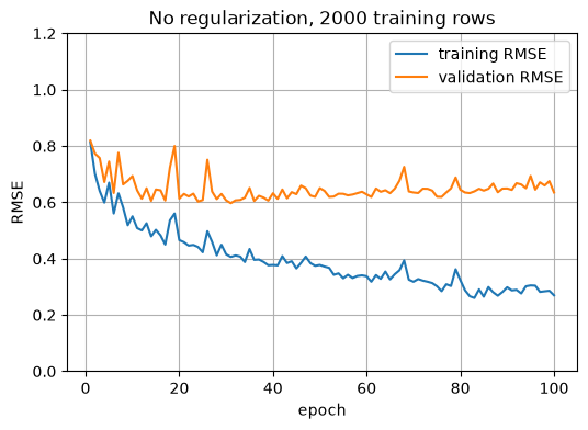
Look at the two columns. The training RMSE keeps going down, from 0.466 at epoch 20 to 0.2698 at epoch 100. The validation RMSE does not follow it. It is 0.6135 at epoch 20 and 0.6353 at epoch 100. Let’s plot every epoch.
# RUN THIS. The training and validation learning curves.epochs =range(1, 101)plt.figure(figsize=(6, 4))plt.plot(epochs, train_rmse_plain, label="training RMSE")plt.plot(epochs, valid_rmse_plain, label="validation RMSE")plt.xlabel("epoch")plt.ylabel("RMSE")plt.ylim(0, 1.2)plt.title("No regularization, 2000 training rows")plt.legend()plt.grid()plt.show()
This is what overfitting looks like in a neural network! At first the two curves are close together, and then they separate. The training curve keeps going down because the network is memorizing the 2000 training rows, including their noise. The validation curve stops going down after the first few dozen epochs and starts to bounce around and creep up, because memorizing the training rows does not help with new rows.
Where was the validation RMSE at its best?
# RUN THIS. Which epoch had the best validation RMSE?best_epoch = np.argmin(valid_rmse_plain) +1# argmin gives the position of the smallest number, +1 because epochs start at 1print("best epoch:", best_epoch)print("validation RMSE at the best epoch:", round(valid_rmse_plain[best_epoch -1], 4))print("validation RMSE after 100 epochs: ", round(valid_rmse_plain[-1], 4))print("training RMSE after 100 epochs: ", round(train_rmse_plain[-1], 4))
best epoch: 31
validation RMSE at the best epoch: 0.5972
validation RMSE after 100 epochs:  0.6353
training RMSE after 100 epochs:    0.2698
The best validation RMSE was 0.5972, at epoch 31. After 100 epochs it was 0.6353. So the last 69 epochs made the model look better on the training rows (0.2698) and worse on new rows.
NOTE - Last class, with all 15,480 training rows, the same kind of network got a validation RMSE of 0.537. More data is the best fix for overfitting, when you can get it. Today we pretend we can’t get more data, so we need some other tools.
NoteQ1. Write this one out by hand
a. In the plot, the training RMSE keeps going down but the validation RMSE does not. In your own words, what is the network doing during those later epochs?
b. Why did we use only 2000 training rows today?
Early Stopping - Stop When the Validation Error Stops Improving
If the best model was at epoch 31, why not just keep that one? That is early stopping: while we train, we check the validation RMSE after every epoch, we keep a copy of the weights from the best epoch, and we stop when the validation RMSE has not improved for a while. We have seen this before! On Day 7 XGBoost did early stopping for us with early_stopping_rounds=50: it kept adding trees until 50 trees in a row failed to improve the validation score, and then kept the best one. Today the “steps” are epochs instead of trees, and we write it ourselves.
There are two new ideas in the code:
Saving the weights.model.state_dict() holds every weight and bias in the model. copy.deepcopy() makes a real copy of it, so the copy does not change as we keep training. At the end, model.load_state_dict() puts the saved weights back.
Patience. The validation RMSE bounces around, so one bad epoch does not mean we are done. The patience is how many epochs in a row we are willing to wait for a new best before we stop. Here we use 20.
# UNDERSTAND THESE STEPS. Early stopping: keep the best weights, stop when validation stops improving.torch.manual_seed(42)model = make_model()optimizer = torch.optim.Adam(model.parameters(), lr=0.001)torch.manual_seed(42) # the same batch order as train_model, so we can compare to the run abovetrain_loader = DataLoader(train_data, batch_size=32, shuffle=True)loss_fn = nn.MSELoss()patience =20# how many epochs we wait for the validation RMSE to improvebest_rmse =float("inf") # the best validation RMSE so far (start at infinity, so anything beats it)best_weights =None# a copy of the weights at the best epochepochs_without_improving =0for epoch inrange(200): # the most epochs we are willing to train model.train()for X_batch, y_batch in train_loader: optimizer.zero_grad() y_pred = model(X_batch) loss = loss_fn(y_pred, y_batch) loss.backward() optimizer.step() model.eval()with torch.no_grad(): rmse = torch.sqrt(loss_fn(model(X_valid_t), y_valid_t)).item()if rmse < best_rmse: # a new best! best_rmse = rmse best_epoch = epoch +1 best_weights = copy.deepcopy(model.state_dict()) # save a copy of every weight and bias epochs_without_improving =0else: # not better than the best so far epochs_without_improving = epochs_without_improving +1if epochs_without_improving == patience: # we waited long enoughprint("stopped after epoch", epoch +1)breakmodel.load_state_dict(best_weights) # put the best weights back in the modelprint("best epoch:", best_epoch, " validation RMSE:", round(best_rmse, 4))
stopped after epoch 51
best epoch: 31   validation RMSE: 0.5972
It found the same best epoch, 31, with the same validation RMSE, 0.5972. Then it waited 20 more epochs for something better, nothing came, and it stopped after epoch 51. We got the best model AND we saved ourselves 49 epochs of training!
BEWARE! Early stopping uses the validation set to decide when to stop, so the validation RMSE of the best epoch is a little bit optimistic. That is one more reason to keep a test set that you only use once, at the very end.
NoteQ2. Write this one out by hand
a. Why can you not do early stopping by watching the training RMSE?
b. What does the patience do? What could go wrong if the patience was 1?
Dropout - Randomly Turning Off Neurons While Training
Early stopping just decides when to stop training. Dropout is different, it changes how the network trains.
A dropout layer goes after an activation function. At every training step, it sets each neuron’s output to 0 with probability p, called the dropout rate. A different random set of neurons is turned off at every step. Usually p is between 0.1 and 0.5.
While training, a different random set of neurons is dropped at every step. When we predict, every neuron is on.
Why would that help? Since any neuron might disappear at any step, the network can not count on one special neuron to memorize a training row. It has to spread what it learns across many neurons, and that usually means it does better on new data.
When we predict, we want the whole network, so dropout turns off in prediction mode. Similar to batch normalization last class, we want our model to act differently in model.train() and model.eval().
In PyTorch, dropout is one more layer in the nn.Sequential: nn.Dropout(p=0.2), right after each nn.ReLU(). Let’s train our network with dropout, everything else the same. Here is the whole network written out, so you can see exactly where the dropout layers go.
# RUN THIS. The same network with a dropout layer after each ReLU.torch.manual_seed(42)dropout_model = nn.Sequential( nn.Linear(8, 100), nn.ReLU(), nn.Dropout(p=0.2), # hidden layer 1, then dropout nn.Linear(100, 100), nn.ReLU(), nn.Dropout(p=0.2), # hidden layer 2, then dropout nn.Linear(100, 100), nn.ReLU(), nn.Dropout(p=0.2), # hidden layer 3, then dropout nn.Linear(100, 1)) # output layer, no dropout here!for layer in dropout_model: # Kaiming initialization from Day 11ifisinstance(layer, nn.Linear): nn.init.kaiming_normal_(layer.weight, nonlinearity="relu") nn.init.zeros_(layer.bias)dropout_optimizer = torch.optim.Adam(dropout_model.parameters(), lr=0.001)train_rmse_dropout, valid_rmse_dropout = train_model(dropout_model, dropout_optimizer, n_epochs=100)
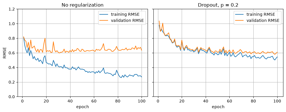
Now compare the two networks and look at the learning curve. Before you look at the graphs… what would we expect to see if our model has stopped overfitting? Make a prediction.
# RUN THIS. The learning curves with and without dropout, side by side.fig, axes = plt.subplots(1, 2, figsize=(10, 4), sharey=True) # sharey=True puts both plots on the same y axisaxes[0].plot(epochs, train_rmse_plain, label="training RMSE")axes[0].plot(epochs, valid_rmse_plain, label="validation RMSE")axes[0].set_title("No regularization")axes[1].plot(epochs, train_rmse_dropout, label="training RMSE")axes[1].plot(epochs, valid_rmse_dropout, label="validation RMSE")axes[1].set_title("Dropout, p = 0.2")for ax in axes: # the same settings on both plots ax.set_xlabel("epoch") ax.set_ylim(0, 1.2) ax.legend() ax.grid()axes[0].set_ylabel("RMSE")plt.tight_layout()plt.show()print("no regularization, after 100 epochs: train", round(train_rmse_plain[-1], 4), " valid", round(valid_rmse_plain[-1], 4))print("dropout 0.2, after 100 epochs: train", round(train_rmse_dropout[-1], 4), " valid", round(valid_rmse_dropout[-1], 4))
no regularization, after 100 epochs:  train 0.2698   valid 0.6353
dropout 0.2, after 100 epochs:        train 0.5435   valid 0.6079
With dropout the two curves stay much closer together. After 100 epochs:
training RMSE
validation RMSE
no regularization
0.2698
0.6353
dropout, p = 0.2
0.5435
0.6079
The training RMSE with dropout is much worse! Even though that feels like maybe it is a bad thing… that is exactly what we want! Dropout makes it hard for the network to memorize the training rows. The validation RMSE is better, 0.6079 against 0.6353, and the gap between training and validation went from about 0.37 to about 0.06.
Notice that dropout also makes the network learn more slowly. It needs more epochs to reach its best validation RMSE, so it is a good idea to use dropout and early stopping together.
NoteQ3. Write this one out by hand
a. In your own words, what does a dropout layer do while the network is training?
b. Why do we turn dropout off (model.eval()) when we predict?
Weight Decay - Ridge Regression for Neural Networks
There is one more tool that you already know. On Day 3, ridge regression added a penalty for big weights to the cost function, so the model could not use huge weights to fit the noise. The same idea works for a neural network, and PyTorch calls it weight decay. It is one argument to the optimizer:
where \lambda is the weight_decay number. The first part says “fit the data”. The second part says “but keep the weights small”. Big weights now cost something, so the network only uses a big weight when it really helps the fit. This is exactly the ridge penalty from Day 3.
NOTE - The loss function is OUR choice! The network learns whatever makes the loss small, so if we change the loss, we change what it learns. Adding a penalty is one way. People also write their own losses, eg. counting some mistakes as worse than others, when that matters for the problem.
NoteQ4. Write this one out by hand
a. Name three ways to fight overfitting in a neural network that we have seen, counting more data. For each one, say in one sentence how it helps.
b. You train a network and the training RMSE is much smaller than the validation RMSE. What does that tell you, and which tool would you try first?
Putting It Together
What this looks like in real life - Dropout and Early Stopping in One Cell
Okay, let’s put it all together! Here is the whole process in one cell, with no helper functions. It uses dropout and early stopping, and the comments show the places you could change things.
# LEARN TO WRITE THIS.# A network with dropout and early stopping, from start to finish.torch.manual_seed(42)# 1. The model. Here you could change the dropout rate, or delete the nn.Dropout linesmodel = nn.Sequential( nn.Linear(8, 100), # 8 features in, 100 neurons nn.ReLU(), nn.Dropout(p=0.2), # dropout after the activation nn.Linear(100, 100), nn.ReLU(), nn.Dropout(p=0.2), nn.Linear(100, 100), nn.ReLU(), nn.Dropout(p=0.2), nn.Linear(100, 1)) # 1 prediction out, no dropout after the output# 2. The starting weightsfor layer in model:ifisinstance(layer, nn.Linear): # only the Linear layers have weights nn.init.kaiming_normal_(layer.weight, nonlinearity="relu") nn.init.zeros_(layer.bias)# 3. The batches, the loss and the optimizertrain_loader = DataLoader(train_data, batch_size=32, shuffle=True)loss_fn = nn.MSELoss()optimizer = torch.optim.Adam(model.parameters(), lr=0.001)# 4. Early stopping. Here you could change the patiencepatience =20best_rmse =float("inf")best_weights =Noneepochs_without_improving =0# 5. The training loopfor epoch inrange(200): # the most epochs we are willing to train model.train() # training mode: dropout is ONfor X_batch, y_batch in train_loader: optimizer.zero_grad() # clear the old gradients y_pred = model(X_batch) # forward pass loss = loss_fn(y_pred, y_batch) # how far off are we? loss.backward() # backward pass optimizer.step() # one step model.eval() # prediction mode: dropout is OFFwith torch.no_grad(): rmse = torch.sqrt(loss_fn(model(X_valid_t), y_valid_t)).item()if rmse < best_rmse: # a new best, save a copy of the weights best_rmse = rmse best_epoch = epoch +1 best_weights = copy.deepcopy(model.state_dict()) epochs_without_improving =0else: epochs_without_improving = epochs_without_improving +1if epochs_without_improving == patience: # no better for 20 epochs in a row, stopprint("stopped after epoch", epoch +1)break# 6. Put the best weights backmodel.load_state_dict(best_weights)print("best epoch:", best_epoch, " validation RMSE:", round(best_rmse, 4))
stopped after epoch 135
best epoch: 115   validation RMSE: 0.5743
With dropout the network learns more slowly, so early stopping let it keep going much longer: the best epoch was 115, and it stopped after epoch 135. The validation RMSE, 0.5743, is the best we got today.
Here is everything from today, all with 2000 training rows:
how we trained it
validation RMSE
no regularization, 100 epochs
0.6353
no regularization, early stopping (best epoch 31)
0.5972
dropout 0.2, 100 epochs
0.6079
dropout 0.2 and early stopping (best epoch 115)
0.5743
NoteQ5. Write this one out by hand
a. In the last cell, why does model.train() come before the batches and model.eval() come before we check the validation RMSE?
b. Why did the network with dropout need many more epochs before early stopping stopped it?
Here is a summary of everything we did today:
Overfitting in a neural network shows up in the learning curves: the training RMSE keeps going down while the validation RMSE stops going down or goes back up.
More data is the best fix, when you can get it.
Early stopping checks the validation RMSE every epoch, keeps a copy of the best weights, and stops after patience epochs with no improvement.
Dropout turns off a random set of neurons at every training step, so the network can not memorize with a few special neurons. It goes after the activation, and it is off in prediction mode.
Weight decay is ridge regression for neural networks: weight_decay= in the optimizer.
model.train() before training and model.eval() before predicting. Every time.
New Commands Today
Command
What it does
The thing that trips people up
nn.Dropout(p=0.2)
a dropout layer, each output is set to 0 with probability p while training
it goes after the activation, and it only works in training mode
model.state_dict()
all the weights and biases of the model
it changes as you train, so save a copy
copy.deepcopy(x)
a real copy of x that will not change when x changes
you need import copy
model.load_state_dict(weights)
puts saved weights back into the model
the model has to have the same layers as when you saved them
np.argmin(my_list)
the position of the smallest number in a list
positions start at 0, epochs start at 1
float("inf")
infinity, bigger than any number
handy as a starting “best so far”
torch.optim.Adam(..., weight_decay=0.0001)
Adam with weight decay (ridge)
small numbers like 0.0001 are typical
TipYou Try: optional code
These are not collected, but they are a great way to practice!
1. In the last cell, change the dropout rate to 0.5. Does it do better or worse? How many epochs does it take?
2. Delete the nn.Dropout lines and add weight_decay=0.0001 to the optimizer instead. How does it compare?
3. Change the patience to 5. Does early stopping stop too soon?
Before Next Class
In your lecture notes notebook, add your handwritten notes and answers to the questions.
Do the Day 13 practice problems in HW_day13.ipynb. They are practice, not graded, and Weekly Homework 7 assumes you have done them. The solutions are in HW-day13-solutions.ipynb.
Weekly Homework 7 is due Sunday 11/8 at 11:59pm. It covers Day 13 and Day 14.
Final project: more about the teams and the proposal soon.
Day 14 is Tuesday 11/3: Convolutional Neural Networks. Read Geron chapter 12, the sections Convolutional Layers and Pooling Layers.
Answers to the Q Boxes
Try every one of these by hand first. These are short summaries. Writing out your own answers is how you really learn this, so give each one a try before you look!
NoteQ1. Overfitting
a. It is memorizing the training rows, including their noise. That makes the training RMSE smaller, but it does not help with new rows, so the validation RMSE stops improving and creeps back up.
b. A big network with only 2000 rows to learn from has lots of room to memorize them, so the overfitting is easy to see. With all 15,480 rows it is much harder to see.
NoteQ2. Early stopping
a. The training RMSE keeps going down almost forever, even while the model is getting worse on new data, so it never tells you to stop. Only the validation RMSE shows when the model stops getting better on new rows.
b. The patience is how many epochs in a row we wait for a new best validation RMSE before we stop. The validation RMSE bounces around, so with a patience of 1 we would stop at the first bad epoch, probably long before the real best epoch.
NoteQ3. Dropout
a. At every training step it sets the output of each neuron to 0 with probability p, a different random set every step, and scales up the ones it keeps. The network can not depend on any one neuron, so it has to spread what it learns out.
b. When we predict we want the whole trained network and we want the same answer every time. Random dropout would make the predictions random and weaker.
NoteQ4. Regularization tools
a. More data: harder to memorize. Early stopping: keeps the weights from before the network started memorizing. Dropout: the network can not memorize with a few special neurons. Weight decay is also a fine answer: it keeps the weights small, like ridge.
b. It is overfitting. Early stopping is the easiest first try, because it is free: you keep the best epoch and you train for less time. Dropout is the next thing to try.
NoteQ5. Putting it together
a. In training mode dropout is on, and that is what we want while we train. In prediction mode dropout is off, so the validation RMSE is computed with the whole network, the same way we would use it for real predictions.
b. Dropout makes the network learn more slowly, because at every step part of it is turned off. Its validation RMSE kept improving for longer, so early stopping kept finding new bests and did not stop until epoch 135.