Blue Q boxes are questions for you to answer by hand, in a notebook, with a pen. Not because I am old fashioned. Writing something down by hand is slow, and slow is the point: it is very hard to write an explanation you do not actually understand. You are welcome to use AI in this class for the mechanics of code, but these boxes are the part where you do the thinking yourself. Bring your written notes to class, I will ask to see them.
Green You Try boxes are optional code for you to work through. Nothing is collected and nothing is graded. They are there because you will learn more from changing a number and rerunning than from watching me do it.
Reading: Geron, chapter 4, the section on Regularized Linear Models
The last part of that section is about Early Stopping. Read it if you like, but we are not doing it today. It only makes sense once you know how gradient descent works, so we come back to it on Day 13, after we have written a training loop by hand.
Last time we found two ways for a model to be wrong. A straight line through a curve was too simple to follow the data, and a degree 300 polynomial was too complicated, it worked to memorize the noise. Today we give those two failures their real names, bias and variance, and then we learn the main tool for controlling them, regularization. The idea behind it is a little strange the first time you see it. We deliberately make the model worse at fitting the training data, on purpose, in exchange for it doing better on data it has not seen. This is almost always a good idea, and regularization shows up again and again in every unit of this class. When we get to neural networks we will use the same idea under different names.
The Same Data as Last Time
We are keeping the Day 2 data so you can compare directly. Same true function, same noise, same seed.
y = \frac{x^2}{2} + x + 2 + \text{noise}
import numpy as npimport matplotlib.pyplot as pltrng = np.random.default_rng(seed=42)m =200# number of data pointsX =6* rng.random((m, 1)) -3# x between -3 and 3y =0.5* X**2+ X +2+ rng.standard_normal((m, 1)) # a parabola plus noiseX_new = np.linspace(-3, 3, 100).reshape(100, 1) # a grid to draw our models on# the true function, which we will plot for comparisondef true_f(x):return0.5* x**2+ x +2print("data shape:", X.shape, y.shape)
data shape: (200, 1) (200, 1)
Bias and Variance
Let’s do an experiment!
On Day 2 we collected one dataset and fit one model to it. But your dataset was a random draw. If you had collected on a different day you would have gotten different points, and you would have gotten a different model. So the honest question is not “how good is this one model” but “what happens to my model when the data changes?”
To find out, we do something you cannot do in real life. We generate 25 separate datasets from the same true function, fit a model to each one, and plot all 25 fitted curves on top of each other. Then we can see the spread.
We do it twice, once with a straight line and once with a degree 8 polynomial.
Q1. Write this one out by hand
Before you run the code below, commit to a guess in your notebook.
a. When we fit 25 straight lines to 25 different samples of the same parabola, will those 25 lines be close to each other or spread far apart?
b. When we fit 25 degree 8 polynomials, will those be close together or spread apart?
c. Which of the two sets of curves do you expect to sit closer to the true parabola on average?
Do not go back and change your guess after you see the answer. Being wrong here is useful.
from sklearn.linear_model import LinearRegression, Ridgefrom sklearn.preprocessing import PolynomialFeatures, StandardScalerdef fit_and_predict(degree, X_train, y_train, X_test, alpha=None):"""Fit a polynomial model of the given degree and predict on X_test. If alpha is None we use plain LinearRegression. If alpha is a number we use Ridge, which we get to later in these notes. """# Step 1: build the polynomial features poly_features = PolynomialFeatures(degree=degree, include_bias=False) X_poly = poly_features.fit_transform(X_train)# Step 2: scale them scaler = StandardScaler() X_scaled = scaler.fit_transform(X_poly)# Step 3: choose the model and fit itif alpha isNone: model = LinearRegression()else: model = Ridge(alpha=alpha) model.fit(X_scaled, y_train)# Step 4: put the test data through the SAME two transforms, then predict.# Note .transform() and not .fit_transform() here. X_test_poly = poly_features.transform(X_test) X_test_scaled = scaler.transform(X_test_poly)return model.predict(X_test_scaled)
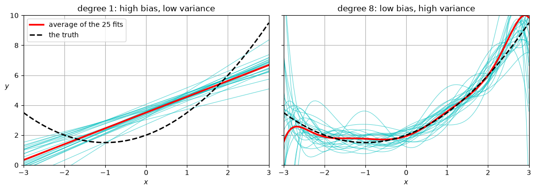
n_samples =25# how many separate datasets we generaten_points =30# how many points in each onecurves = {1: [], 8: []}for trial inrange(n_samples):# a fresh random dataset from the same true function r = np.random.default_rng(seed=100+ trial) X_sample =6* r.random((n_points, 1)) -3 y_sample = true_f(X_sample) + r.standard_normal((n_points, 1))for degree in curves: y_pred = fit_and_predict(degree, X_sample, y_sample, X_new) curves[degree].append(y_pred.ravel())fig, axes = plt.subplots(1, 2, figsize=(11, 4), sharey=True)titles = ["degree 1: high bias, low variance", "degree 8: low bias, high variance"]for ax, degree, title inzip(axes, [1, 8], titles):for one_curve in curves[degree]: ax.plot(X_new, one_curve, "c-", linewidth=0.8, alpha=0.6) ax.plot(X_new, np.mean(curves[degree], axis=0), "r-", linewidth=2.5, label="average of the 25 fits") ax.plot(X_new, true_f(X_new), "k--", linewidth=2, label="the truth") ax.set_title(title); ax.set_xlabel("$x$"); ax.grid(); ax.axis([-3, 3, 0, 10])axes[0].set_ylabel("$y$", rotation=0); axes[0].legend()plt.tight_layout()plt.show()
Look at the left panel first. The 25 cyan lines are all basically on top of each other. Change the data and you get almost the same line back. But the red average of those lines is not the parabola, it is a line, and it misses the truth badly on the left side. The model is stable but wrong.
Now the right panel. The red average sits almost exactly on the black dashed truth, so on average degree 8 has the right shape. But the individual cyan curves wander all over, especially out near the edges where there are fewer points. Any one of those curves is a bad model, even though their average is good. The model is right on average but unstable.
Those two failures have names.
Bias is how far off you are on average over many datasets. High bias means the model is too simple to represent the pattern, so it is wrong in the same direction no matter what data you hand it. This is underfitting from Day 2. We could measure this by comparing the average of all the curves and the real curve.
Variance is how much your model moves around when the data changes. High variance means the model is chasing the particular noise in the particular sample you got. This is overfitting from Day 2. We could measure this by finding the variance in the data for each of the curves and then averaging it.
NOTE: np.var() used below calculates the population variance by default
VAR = \frac{\sum (x_i - \bar{x})^2}{N}
where N is the number of samples.
for degree in [1, 8]: all_curves = np.array(curves[degree]) # 25 rows, one per fitted model average_curve = all_curves.mean(axis=0)# bias squared: how far the AVERAGE model is from the truth bias_squared = np.mean((average_curve - true_f(X_new).ravel())**2)# variance: how much the individual models spread around their own average variance = np.mean(all_curves.var(axis=0))print(f"degree {degree}:")print(f" bias squared = {bias_squared:.3f}")print(f" variance = {variance:.3f}")print(f" sum = {bias_squared + variance:.3f}")
What you notice is that one example is high bias and low variance and the other is opposite. They switch places!
bias squared
variance
degree 1
1.884
0.220
degree 8
0.189
3.261
Going from degree 1 to degree 8 cut the bias by a factor of about 10 and raised the variance by a factor of about 15. Neither model is good. Degree 1 is bad because it is wrong, degree 8 is bad because it is unstable.
This is the bias variance tradeoff, and the reason it is called a tradeoff is that with a fixed amount of data you usually cannot lower both at once. Making a model more flexible lowers bias and raises variance. Making it simpler does the opposite. Your total expected error is roughly
and that last term is the noise in the data itself, which you cannot do anything about. In our case we added noise with a standard deviation of 1.0 on purpose, so no model, no matter how clever, can get its RMSE below about 1.0 here. Keep that in mind when we start comparing scores later.
Q2. Write this one out by hand
a. In your own words, what is the difference between a model with high bias and a model with high variance? Do not use the words underfitting or overfitting in your answer.
b. In the right hand plot, the individual curves are worst near x = -3 and x = 3 and best near the middle. Why? What is different about the edges?
c. We could only run this experiment because we made the data ourselves and could generate 25 fresh datasets. With real data you get one dataset. So how would you detect high variance in real life? Name something specific you learned on Day 2.
Q3. Write this one out by hand
Suppose you collected 10 times as much data, so 300 points in each sample instead of 30, and reran the whole experiment.
a. What do you expect to happen to the variance of the degree 8 fits? Why?
b. What do you expect to happen to the bias of the degree 1 fits? Why?
c. Based on your two answers, is “collect more data” a fix for high bias, high variance, both, or neither?
Okay so what do we want? We want a flexible model (low bias) but we want the model to not be able to do so much memorization (less variance). This is what regularization does! Ridge, Lasso, and Elastic Net Regression are each types of regularization that add a term to the cost function, aka the thing we are minimizing.
Ridge Regression
So we want the low bias of a flexible model without the wild variance that comes with it. Here is the trick.
Go back to what a linear model is actually doing. It assumes a linear model
\hat{y} = w_0 + w_1 X_1 + w_2 X_2 + \dots
then it picks weights w_1, w_2, \dots, w_n to make the mean squared error as small as possible:
Nothing in that formula says the weights have to be reasonable. If the model can drive the error down a little by using a weight of 2000, it will, and that is exactly how you get those crazy wiggly curves. A curve that swings up and down violently between the data points is a curve with enormous weights. You could experiment with this yourself… make a plot of a polynomial y=ax^2+bx+c and see what happens when a, b, and c are big vs small.
Ridge regression adds a second term that penalizes the model for big weights:
Now the model has to balance two things it wants. It still wants low error, but every weight it uses costs it something. The number \alpha (alpha) sets the balance between them, and it is yours to choose.
\alpha = 0 means the penalty is free, and you are back to plain linear regression.
Small \alpha means a mild nudge toward smaller weights.
Large \alpha means the model cares much more about small weights than about fitting your data, and in the limit as \alpha gets large, it pushes every weight to zero and just predicts the mean.
A number like \alpha that you choose yourself, rather than something the model learns from the data, is called a hyperparameter. You will hear that word constantly for the rest of the semester.
Q4. Write this one out by hand
Look at the Ridge cost function above.
a. What happens to the fitted model as \alpha gets very large, say a million? Describe the shape of the curve you would get, and say why the math forces that.
b. Notice that the penalty adds up w_i^2 for i=1 and higher, so it never charges the model for the intercept, only for the slopes. Why would it be a bad idea to penalize the intercept too?
c. Ridge asks the model to keep its weights small. Explain in one or two sentences why small weights and a smooth, not very wiggly curve are the same thing.
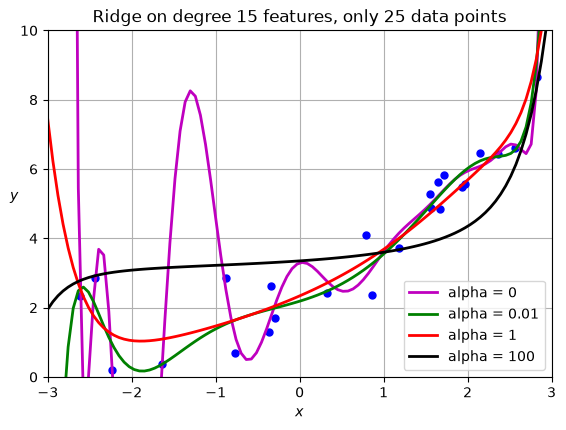
Below we fit degree 15 polynomials with four different values of \alpha. Notice that we are only using 25 data points here, not all 200. This helps us to really highlight the effect of regularization… more data is a type of regularization in itself.
# only the first 25 points, so that overfitting is actually a problemX_few = X[:25]y_few = y[:25]plt.figure(figsize=(6.5, 4.5))plt.plot(X_few, y_few, "b.", markersize=10)for alpha, style inzip([0, 0.01, 1, 100], ["m-", "g-", "r-", "k-"]):# alpha = 0 means no penalty at all, so use plain LinearRegressionif alpha ==0: y_pred = fit_and_predict(15, X_few, y_few, X_new, alpha=None)else: y_pred = fit_and_predict(15, X_few, y_few, X_new, alpha=alpha) plt.plot(X_new, y_pred, style, linewidth=2, label=f"alpha = {alpha}")plt.xlabel("$x$"); plt.ylabel("$y$", rotation=0)plt.axis([-3, 3, 0, 10]); plt.legend(); plt.grid()plt.title("Ridge on degree 15 features, only 25 data points")plt.show()
The purple curve, with no penalty at all, is the Day 2 disaster again. It runs off the top of the plot twice and dives to the bottom in between, all so it can pass close to 25 points.
The green curve, alpha 0.01, is much calmer but still chasing individual points.
The red curve, alpha 1, is close to the parabola we know is the right answer, and it got there without us telling it the degree was wrong. Think about what happened here. We handed the model 15 features it did not need, and regularization let it decline to use them.
The black curve, alpha 100, has gone too far the other way. The penalty now dominates and the model is nearly a straight line. We decreased the variance too far and ended up with high bias (a bad model)
Q5. Write this one out by hand
Compare the black curve here to the straight line from Day 2.
a. Both are close to straight, but they got there in completely different ways. Explain the difference.
b. If you were handed only the black curve and told “this model is underfitting”, what would you change to fix it? Be specific about which number you would change and which direction you would move it.
Scaling Is Not Optional Here
First, what does StandardScaler actually do?
We have been using it since Day 2 without ever saying what it is. It is simpler than the name makes it sound.
For each feature, on its own, it subtracts the mean and divides by the standard deviation:
z = \frac{x - \text{mean}}{\text{standard deviation}}
So every feature comes out with a mean of 0 and a standard deviation of 1. A value of z = 2 means “two standard deviations above average for this feature”, whatever the feature was measured in.
Say you have house prices around 400,000 dollars and bedroom counts around 3. After scaling, both columns are centered on 0 and both spread out by about 1. The dollars and the bedrooms are now on the same footing, and the model can compare them.
Two things worth knowing:
It does not change the shape of your data. A histogram of a scaled feature looks exactly like the original, just with different numbers on the axis.
The mean and standard deviation it uses come from .fit(). That is why we always .fit_transform() the training data and only .transform() everything else, which is the habit we come back to at the end of this section.
Why it matters more once you regularize
On Day 2 we scaled the features because x^{300} is an enormous number and the arithmetic fell apart without it. With regularization there is a second, more important reason.
The penalty \alpha \sum w_i^2 charges the model per unit of weight, and it charges every feature at the same rate. But if one of your features is measured in thousands and another in hundredths, the weights that go with them are on wildly different scales, and the same penalty hits them very differently. The feature with the big numbers gets a tiny weight and is barely penalized. The feature with small numbers needs a huge weight to matter, and gets crushed.
So the penalty ends up depending on the units your variables happened to be measured in, which is not a property you want your model to have.
Always scale your features before you regularize. Here is an example that shows just what happens when you don’t scale your data!
from sklearn.model_selection import train_test_splitfrom sklearn.metrics import root_mean_squared_errorX_train, X_valid, y_train, y_valid = train_test_split( X, y, test_size=0.3, random_state=42)print("training points :", len(X_train))print("validation points:", len(X_valid))# Step 1: build the degree 15 features once, from the training data onlypoly_features = PolynomialFeatures(degree=15, include_bias=False)X_train_poly = poly_features.fit_transform(X_train)X_valid_poly = poly_features.transform(X_valid)# Step 2: scale them, again learning the scaling from the training data onlyscaler = StandardScaler()X_train_scaled = scaler.fit_transform(X_train_poly)X_valid_scaled = scaler.transform(X_valid_poly)# now fit the same Ridge model both waysridge_unscaled = Ridge(alpha=1.0)ridge_unscaled.fit(X_train_poly, y_train)rmse_unscaled = root_mean_squared_error(y_valid, ridge_unscaled.predict(X_valid_poly))ridge_scaled = Ridge(alpha=1.0)ridge_scaled.fit(X_train_scaled, y_train)rmse_scaled = root_mean_squared_error(y_valid, ridge_scaled.predict(X_valid_scaled))print("\nRidge alpha = 1 on degree 15 features")print(" features not scaled: validation RMSE =", round(rmse_unscaled, 3))print(" features scaled : validation RMSE =", round(rmse_scaled, 3))
training points  : 140
validation points: 60

Ridge alpha = 1 on degree 15 features
  features not scaled: validation RMSE = 1.113
  features scaled    : validation RMSE = 0.97
Unscaled gives 1.113 and scaled gives 0.970, so forgetting the scaler cost about 15 percent of accuracy on a model where everything else was identical. That is not catastrophic in this case, but it is free to avoid, and on real data it can be much worse. Always scale your data!
Notice the other thing in that code, because it is the habit that matters most in this whole class. We called .fit_transform() on the training data and .transform() on the validation data. The scaler learned its mean and standard deviation from the training set only. If we had called .fit_transform() on the validation set too, the model would have gotten a peek at data it is supposed to be tested on. That is called leakage, and it is the whole subject of Day 4.
Choosing Alpha
We now have a hyperparameter and no idea what to set it to. So we try a lot of values and look at what happens to the training and the validation error for each one.
Below we try 40 values of \alpha spread across nine orders of magnitude, from 0.00001 up to 10000. np.logspace(-5, 4, 40) gives us 40 values spaced evenly on a log scale, which is the right way to search a hyperparameter that could plausibly be any size.
alpha_list = np.logspace(-5, 4, 40) # 40 values from 1e-5 to 1e4train_rmse = []valid_rmse = []for alpha in alpha_list: model = Ridge(alpha=alpha) model.fit(X_train_scaled, y_train) train_rmse.append(root_mean_squared_error(y_train, model.predict(X_train_scaled))) valid_rmse.append(root_mean_squared_error(y_valid, model.predict(X_valid_scaled)))# which alpha did best on the validation set?best = np.argmin(valid_rmse)print("best alpha =", round(alpha_list[best], 4))print(" training RMSE =", round(train_rmse[best], 3))print(" validation RMSE =", round(valid_rmse[best], 3))print()print("almost no penalty, alpha =", round(alpha_list[0], 5))print(" training RMSE =", round(train_rmse[0], 3))print(" validation RMSE =", round(valid_rmse[0], 3))print()print("far too much penalty, alpha =", round(alpha_list[-1], 1))print(" training RMSE =", round(train_rmse[-1], 3))print(" validation RMSE =", round(valid_rmse[-1], 3))plt.figure(figsize=(6.5, 4.5))plt.semilogx(alpha_list, train_rmse, "r-+", linewidth=2, label="training set")plt.semilogx(alpha_list, valid_rmse, "b-", linewidth=2.5, label="validation set")plt.axvline(alpha_list[best], color="k", linestyle=":", label=f"best alpha = {alpha_list[best]:.3f}")plt.xlabel("alpha (log scale)"); plt.ylabel("RMSE")plt.title("Too little regularization, too much, and just right")plt.legend(); plt.grid(); plt.ylim(0, 3)plt.show()
best alpha      = 1.1938
  training RMSE   = 0.998
  validation RMSE = 0.97

almost no penalty, alpha = 1e-05
  training RMSE   = 0.984
  validation RMSE = 1.149

far too much penalty, alpha = 10000.0
  training RMSE   = 2.362
  validation RMSE = 2.186
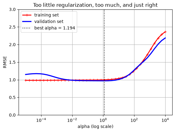
Read that plot from left to right.
On the far left the penalty is almost nothing. The training error is at its lowest, 0.984, and the validation error is at 1.149, above it. That gap is the overfitting signature from Day 2, really good on the training set much less good on the validation set, a model that is memorizing the training data.
In the middle the two curves come together and the validation error bottoms out at 0.970 with \alpha around 1.19. Remember that the noise we added has a standard deviation of 1.0, so 0.970 is about as good as anything can do on this data. The model with 15 useless features and the right amount of regularization is performing like the model that knew the answer was a parabola.
On the far right both errors climb together, to 2.362 and 2.186. Too much penalty and the model underfits. Both curves high and close together, which is exactly what Day 2 told us underfitting looks like, really bad on the training really bad on the validation, just a bad model.
One detail that surprises people: on the right side the validation error is slightly lower than the training error, 2.186 against 2.362. That is not a mistake, but it is also not good news. When a model is badly underfitting it is equally bad everywhere, and which of two random subsets it happens to be slightly less bad on is luck. Only 60 validation points are involved.
Q6. Write this one out by hand
a. The training error curve only ever goes up as \alpha increases, never down. Explain why that has to be true, from the cost function.
b. The validation curve goes down and then back up. Explain what is causing each half of that U shape.
c. We picked our \alpha by choosing whichever value scored best on the validation set. Day 1 said you only get to use your test set once. Explain why what we just did is allowed with a validation set, and what would have gone wrong if we had used the test set for this.
One split is a shaky way to choose
We picked alpha = 1.19 based on 60 validation points. Had train_test_split handed us a different 60, we would have picked a somewhat different alpha.
Scikit-learn has RidgeCV, which does this search using cross validation instead of a single split, and it is what you should actually use. We are holding off on it for one class because cross validation deserves a full day of its own, and that is Day 4.
Lasso Regression
Lasso does the same thing as Ridge with one small change to the penalty. Instead of squaring the weights, it uses their absolute values:
That small change makes a big difference in how the model behaves, and you can see it immediately.
Ridge shrinks all the weights toward zero, but almost never all the way to zero. Lasso pushes some weights exactly to zero, and leaves the rest alone. A weight of exactly zero means the feature is not being used at all, so Lasso does not just shrink your model, it throws features out. That is called producing a sparse model, and it is why people reach for Lasso when they have a pile of features and suspect most of them are junk.
Watch it happen. We give both models the same 15 polynomial features and count how many survive.
from sklearn.linear_model import Lassoprint("Lasso, how many of the 15 weights are not zero:")for alpha in [0.0001, 0.01, 0.1, 1.0]: model = Lasso(alpha=alpha, max_iter=100000) model.fit(X_train_scaled, y_train.ravel()) n_used = np.sum(np.abs(model.coef_) >1e-8) rmse = root_mean_squared_error(y_valid, model.predict(X_valid_scaled))print(f" alpha = {alpha:<8} weights used = {n_used:2d}/15 validation RMSE = {rmse:.3f}")print("\nRidge on the exact same features:")for alpha in [0.0001, 0.01, 1.0, 100.0]: model = Ridge(alpha=alpha) model.fit(X_train_scaled, y_train) n_used = np.sum(np.abs(model.coef_) >1e-8) rmse = root_mean_squared_error(y_valid, model.predict(X_valid_scaled))print(f" alpha = {alpha:<8} weights used = {n_used:2d}/15 validation RMSE = {rmse:.3f}")
Lasso, how many of the 15 weights are not zero:
  alpha = 0.0001    weights used = 10/15   validation RMSE = 0.993
  alpha = 0.01      weights used =  3/15   validation RMSE = 0.962
  alpha = 0.1       weights used =  3/15   validation RMSE = 0.974
  alpha = 1.0       weights used =  2/15   validation RMSE = 1.684

Ridge on the exact same features:
  alpha = 0.0001    weights used = 15/15   validation RMSE = 1.167
  alpha = 0.01      weights used = 15/15   validation RMSE = 0.985
  alpha = 1.0       weights used = 15/15   validation RMSE = 0.970
  alpha = 100.0     weights used = 15/15   validation RMSE = 1.276
Ridge uses all 15 weights at every value of alpha. Lasso at alpha 0.01 gets down to 3 weights out of 15 and scores 0.962 on the validation set, which is the best number we have seen today.
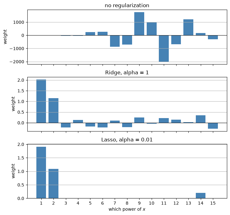
Let’s look at the actual weights, the picture is easier to read than the table.
# three models on identical featuresplain_model = LinearRegression()plain_model.fit(X_train_scaled, y_train)ridge_model = Ridge(alpha=1.0)ridge_model.fit(X_train_scaled, y_train)lasso_model = Lasso(alpha=0.01, max_iter=100000)lasso_model.fit(X_train_scaled, y_train.ravel())powers = np.arange(1, 16)all_coefs = [plain_model.coef_.ravel(), ridge_model.coef_.ravel(), lasso_model.coef_.ravel()]names = ["no regularization", "Ridge, alpha = 1", "Lasso, alpha = 0.01"]fig, axes = plt.subplots(3, 1, figsize=(7.5, 7), sharex=True)for ax, coefs, name inzip(axes, all_coefs, names): ax.bar(powers, coefs, color="steelblue") ax.axhline(0, color="k", linewidth=0.8) ax.set_title(name); ax.grid(axis="y"); ax.set_ylabel("weight")axes[-1].set_xlabel("which power of $x$")axes[-1].set_xticks(powers)plt.tight_layout()plt.show()print("Total size of the weights, adding up absolute values across all 15:")for coefs, name inzip(all_coefs, names):print(f" {name:<22}: {np.abs(coefs).sum():.1f}")
Total size of the weights, adding up absolute values across all 15:
  no regularization     : 9261.0
  Ridge, alpha = 1      : 5.5
  Lasso, alpha = 0.01   : 3.2
Look at the vertical axis on the top panel. With no regularization the weights run into the thousands, positive and negative, and they nearly cancel each other out. Adding them up in absolute value gives 9261. Those huge weights are what the wiggly curve is made of.
Ridge with alpha 1 brings the total down to 5.5. Every weight is still there but they are all small, and the two biggest belong to x and x^2, which is correct.
Lasso with alpha 0.01 brings the total to 3.2 and keeps only three weights: x, x^2, and a small amount of x^{14}. It found the parabola on its own. Nobody told it the answer was degree 2, it worked that out from 140 data points.
The x^{14} term is a good reminder that these methods are useful but not perfect. It is picking up a little bit of noise near the edges of the data. Do not expect a clean answer just because you regularized.
Q7. Write this one out by hand
a. Ridge and Lasso differ only in whether the penalty squares the weights or takes their absolute value. Explain, in words, what that change does to the resulting model.
b. You are predicting house prices and you have 400 features, and you believe only a handful actually matter. Which of the two would you reach for, and why?
c. Now you are predicting house prices from square footage, number of bedrooms, and number of bathrooms. All three certainly matter, and they are strongly related to each other. Which would you reach for now, and why?
d. Lasso at alpha = 1.0 got down to 2 weights but its validation RMSE jumped to 1.684, much worse than at alpha = 0.01. What went wrong? Is a sparser model always a better model?
Elastic Net
If you are torn between the two, Elastic Net is both of them at once. It uses a mix of the two penalties:
There are now two knobs. \alpha still controls how much total penalty you apply, and the mix ratio r controls how much of that penalty is the Lasso kind. In scikit-learn r is called l1_ratio.
l1_ratio = 0 is pure Ridge
l1_ratio = 1 is pure Lasso
anything in between is a blend
The reason this exists is that pure Lasso can behave badly when features are strongly related to each other. If two features carry nearly the same information, Lasso tends to pick one at random and zero out the other, and which one it picks can flip if your data changes slightly. Elastic Net with a bit of Ridge mixed in keeps related features together instead of choosing between them arbitrarily.
from sklearn.linear_model import ElasticNetprint("Elastic Net at alpha = 0.01, changing only the mix:")for l1_ratio in [0.0, 0.25, 0.5, 0.75, 1.0]: model = ElasticNet(alpha=0.01, l1_ratio=l1_ratio, max_iter=100000) model.fit(X_train_scaled, y_train.ravel()) n_used = np.sum(np.abs(model.coef_) >1e-8) rmse = root_mean_squared_error(y_valid, model.predict(X_valid_scaled))print(f" l1_ratio = {l1_ratio:<5} weights used = {n_used:2d}/15 validation RMSE = {rmse:.3f}")
Elastic Net at alpha = 0.01, changing only the mix:
  l1_ratio = 0.0    weights used = 15/15   validation RMSE = 0.970
  l1_ratio = 0.25   weights used =  9/15   validation RMSE = 0.967
  l1_ratio = 0.5    weights used =  7/15   validation RMSE = 0.965
  l1_ratio = 0.75   weights used =  4/15   validation RMSE = 0.963
  l1_ratio = 1.0    weights used =  3/15   validation RMSE = 0.962
The number of weights slides smoothly from 15 down to 3 as we move the mix from pure Ridge to pure Lasso, and the validation RMSE barely budges, from 0.970 to 0.962. On this particular data every setting works about equally well, and that is a genuinely useful thing to notice: a difference of 0.008 RMSE on 60 validation points is not a real difference. Do not go bragging about the third decimal place.
So which one should you use? Our book’s advice, which is good advice:
Regularizing at all beats plain linear regression almost always, so do not use plain LinearRegression as your final model.
Ridge is the sensible default when you think most of your features matter.
Lasso or Elastic Net when you suspect only a few of your features matter, because they will tell you which ones.
Prefer Elastic Net over pure Lasso when you have more features than data points, or when features are strongly related to each other, because Lasso can behave erratically in those cases.
Q8. Write this one out by hand
Every one of the five Elastic Net settings above landed between 0.962 and 0.970 validation RMSE.
a. A classmate says “l1_ratio = 1.0 is the best model, its RMSE is lowest.” What is wrong with that claim?
b. What would you need in order to make an honest claim that one of these settings really is better than another? Think about what changed between our two RMSE numbers, and how many points went into each one.
Why Anyone Cares About a Sparse Model
We have been judging these models by their RMSE, which is the right thing to do most of the time and is not the whole story. Sparsity buys you something that does not show up in the error at all.
A model with 4 features is a model a person can look at. A doctor can read four numbers, decide whether they make clinical sense, and tell you if one of them is obviously wrong. Nobody can do that with 60. That matters more than it sounds like, because a model people trust and actually use beats a slightly more accurate model they ignore. Fewer features also means fewer things to collect, fewer places for missing data to ruin your day, and less to maintain in two years when you have moved on and somebody else is using the model.
So it can be entirely reasonable to have your final model a sparse model that scores a little worse.
Now the catch, and it follows directly from what Elastic Net exists to fix. A feature being dropped is not evidence that the feature does not matter. When several features carry nearly the same information, Lasso keeps one and zeros the others, and which one survives is close to arbitrary. So if you hand a doctor your list of 4 surviving features and tell them “these are the 4 things that predict readmission”, you have said something stronger than your model actually knows, there could be other things that predict readmission pretty well but Lasso dropped them arbitrarily.
And before you put any model anywhere that affects people, there are questions the RMSE cannot answer for you:
Who is hurt when it is wrong, and how badly? Being off by 0.3 on a house price and being off by 0.3 on a hospital readmission risk are not the same kind of mistake.
Is the error spread evenly? An average error hides the possibility that the model is fine for most patients and terrible for one group of them.
Is the difference real? We saw today that 0.962 and 0.970 on 60 validation points is not a real difference. Neither is 0.28 against 0.31 if the validation set is small.
We are going to keep coming back to these, and Day 5 is entirely about the fact that one number is never enough to describe how a model behaves.
Q9. Write this one out by hand
A teammate builds a model to predict which hospital patients will be readmitted within 30 days. They used Lasso with a large alpha, it kept only 4 of 60 features, and they are pleased because doctors can understand it. Their validation RMSE is 0.31. The unregularized model got 0.28.
a. Give one good reason to ship their sparse model anyway, even though its error is higher.
b. Give one reason to be nervous about it. Use what you know about what Lasso does with features that carry similar information.
c. Name two things you would want to know before you agreed to put either model into a hospital.
You Try: optional code
Nothing here is collected. Work through it if you want the idea to stick.
1. Go back to the alpha sweep and change X_train to use only 25 points instead of 140:
X_train_small = X[:25]
y_train_small = y[:25]
Rebuild the features and rerun the sweep. Does the best alpha get bigger or smaller when you have less data? Guess before you run it, then explain what you got.
2. Try Lasso with alpha=0.05 and print out the weights with lasso_model.coef_. Which powers of x does it keep? Does it still find the parabola?
3. Rerun the bias and variance experiment from the top of these notes, but instead of plain LinearRegression for degree 8, use alpha=1. The fit_and_predict function already takes an alpha, so this is a one word change. What happens to the bias number? What happens to the variance number? This is the whole point of today in two numbers.
Before Next Class
In your lecture notes notebook, add your hand written notes and answers to the questions. Short answers are at the very bottom of these notes in drop down boxes, but do the writing first, that is the part that does the work.
Finish the Day 3 practice problems in HW_day3.ipynb. They are part of HW 2, due Sunday 9/13 at 11:59pm, along with the Day 4 problems.
Read Geron chapter 2, the section on Create a Test Set, and chapter 3, the section on Measuring Accuracy Using Cross-Validation.
Watch the Day 4 video on the class website.
Today we chose alpha by looking at how it scored on one validation set of 60 points. That worked, but it is fragile, and we said so at the time. Day 4 fixes it. We will look at cross validation properly, and then at all the ways a train/test split can hand you a number you should not trust. That list is longer than you would expect.
Answers to the Q Boxes
Try every one of these by hand first. These are short summaries, not full answers, and the writing out is the part that does the work. If your answer says the same thing in more words, you are fine.
Q1. The 25 fits
a. Close together. b. Spread far apart, worst near the edges. c. The degree 8 curves. Their average sits almost on the true parabola, while the average straight line cannot bend and misses on the left.
Q2. Bias, variance, and the edges
a. High bias means the model is wrong in the same direction every time, no matter which data you give it. High variance means the answer changes a lot depending on which data you happened to get.
b. There are fewer points near the edges, and nothing outside them to hold the curve down. A flexible model is least constrained there, so that is where it swings.
c. Look at the gap between the training and validation curves on a learning curve. A big gap means high variance.
Q3. Ten times as much data
a. The variance drops a lot. More points pin the curve down, so the 25 fits stop wandering.
b. The bias barely moves. A straight line still cannot bend, and more points on a parabola do not change that.
c. More data fixes high variance. It does not fix high bias.
Q4. Reading the Ridge cost function
a. Every weight gets driven to zero and you get a flat horizontal line at the mean of y. With alpha that large the penalty term is so much bigger than the MSE term that the cheapest thing the model can do is use no weights at all.
b. The intercept only sets the height of the model. Penalizing it would pull your predictions toward zero instead of toward the mean of your data, and zero is not a special number for most datasets.
c. The weights control how fast the curve is allowed to change as x changes. Big weights let it climb and dive quickly, which is what a wiggle is. Small weights limit how fast it can change, so the curve has to be smooth.
Q5. Two ways to be almost straight
a. The Day 2 line had only two parameters and could not bend. The alpha 100 curve has all 15 and is perfectly able to bend, but the penalty makes it choose not to. Same shape, completely different reason.
b. Lower alpha. Underfitting means too much penalty, so move alpha down and refit.
Q6. Reading the alpha sweep
a. Alpha = 0 is by definition the value that makes the training MSE as small as it can be. Any larger alpha spends some of the model’s effort on keeping weights small instead, so the training error can only get worse.
b. Going down on the left: you are removing overfitting. Going up on the right: you are adding underfitting.
c. The validation set exists to be used over and over for choices like this. If you tuned alpha on the test set, the test score would reflect a choice you made using it, so it would no longer be an honest estimate of how you do on brand new data.
Q7. Ridge versus Lasso
a. Squaring shrinks every weight but almost never to exactly zero, so you keep all your features. Absolute value pushes some weights exactly to zero, which drops those features entirely.
b. Lasso. It will shrink most of the 400 to zero and show you the handful that matter.
c. Ridge, or Elastic Net. The three features carry similar information, and Lasso would keep one and zero the other two more or less arbitrarily, which would be misleading.
d. Too much penalty, so the model underfits. No, a sparser model is not automatically better.
Q8. Is the difference real?
a. 0.962 and 0.970 are 0.008 apart on only 60 validation points. That is well inside the wobble you would get from a different random split, so it is not evidence that one setting beats another.
b. Either a lot more validation data, or the same comparison repeated over many different splits so you can see whether the ordering holds up. That is cross validation, and it is Day 4.
Q9. The hospital model
a. Four features is something a doctor can actually read and sanity check, and a model people trust and use beats a slightly better one they ignore. Fewer features also means less data to collect and less to maintain.
b. A dropped feature is not proof that the feature does not matter. Lasso keeps one out of a group of similar features and zeros the rest close to arbitrarily, so something clinically important could have disappeared for a purely statistical reason.
c. Any two of: how big the validation set was, whether 0.28 against 0.31 survives cross validation, which 56 features got dropped and whether a doctor agrees they do not matter, whether the error is spread evenly across patient groups, and what happens to a patient the model gets wrong.