Blue Q boxes are questions for you to answer by hand, in a notebook, with a pen. Not because I am old fashioned. Writing something down by hand is slow, and slow is the point: it is very hard to write an explanation you do not actually understand. You are welcome to use AI in this class for the mechanics of code, but these boxes are the part where you do the thinking yourself. Bring your written notes to class, I will ask to see them.
Green You Try boxes are optional code for you to work through. Nothing is collected and nothing is graded. They are there because you will learn more from changing a number and rerunning than from watching me do it.
Short answers to the Q boxes are in drop down boxes at the very bottom. Write yours first.
Reading: Geron, chapter 2, the section on Create a Test Set, and chapter 3, the section on Measuring Accuracy Using Cross-Validation
On Day 3 we picked alpha by scoring 40 values on one validation set of 60 points, and I said at the time that this was fragile. Today we find out how fragile, and then fix it.
This is the least glamorous day of the semester and it is the one that will save you the most embarrassment. Everything today is about the difference between a number that looks good and a number you can actually trust. Every model in this class from here on gets evaluated with the tools from today.
Three Sets, and the Rule About the Last One
Before anything else, get the vocabulary straight, because people use these words loosely and then confuse each other.
The training set is what the model learns from. It sees this data and fits its weights to it.
The validation set is what you use to make choices. Which alpha, which degree, which model. You are allowed to look at it many times, because you are not fitting weights to it, you are picking between options.
The test set is what you use once, at the very end, to estimate how the finished model will do on data nobody has seen.
The reason the test set is special is worth being precise about. Every time you look at a score and change something because of it, you are fitting to that data a little bit. Do that a hundred times with your validation set and the validation score stops being an honest estimate, which is fine, because that was never its job. But if you do it with your test set, you have nothing left that is honest.
Geron says to create the test set first, before you even look at the data properly, and that advice is not fussiness. If you explore all the data first, you will notice patterns, and the choices you make afterwards will be shaped by things you saw in the test set. Your brain becomes the leak.
Q1. Write this one out by hand
a. In your own words, what is the difference between what a validation set is for and what a test set is for?
b. You try 200 different models and report the validation score of whichever one scored best. Is that number an honest estimate of how the model will do on new data? Why or why not?
c. Geron says to split off the test set before you explore the data. Explain the danger he is protecting you from, in a situation where nothing in your code touches the test set at all.
One Split Is Not Enough
Here is the Day 3 problem, made visible.
We take the same data, and instead of splitting it once, we split it ten different ways and run the whole alpha search each time. If a single split were a reliable way to choose a hyperparameter, all ten runs would pick roughly the same alpha.
Q2. Write this one out by hand
Before running it, guess. Across ten different random splits of the same 200 points, how much do you think the chosen alpha will vary? Within a factor of 2? A factor of 10? More?
Write down a number. Then run it.
import numpy as npimport matplotlib.pyplot as pltfrom sklearn.linear_model import Ridgefrom sklearn.preprocessing import PolynomialFeatures, StandardScalerfrom sklearn.metrics import root_mean_squared_errorfrom sklearn.model_selection import train_test_split# the same data as Day 2 and Day 3rng = np.random.default_rng(seed=42)m =200X =6* rng.random((m, 1)) -3y = (0.5* X**2+ X +2+ rng.standard_normal((m, 1))).ravel()alphas = np.logspace(-3, 3, 25)best_alphas = []best_rmses = []for seed inrange(10):# the ONLY thing that changes between runs is which points land in which set X_train, X_valid, y_train, y_valid = train_test_split( X, y, test_size=0.3, random_state=seed) poly_features = PolynomialFeatures(degree=15, include_bias=False) X_train_poly = poly_features.fit_transform(X_train) scaler = StandardScaler() X_train_scaled = scaler.fit_transform(X_train_poly) X_valid_scaled = scaler.transform(poly_features.transform(X_valid)) rmses = []for alpha in alphas: model = Ridge(alpha=alpha) model.fit(X_train_scaled, y_train) rmses.append(root_mean_squared_error(y_valid, model.predict(X_valid_scaled))) i =int(np.argmin(rmses)) best_alphas.append(alphas[i]) best_rmses.append(rmses[i])print(f" split seed {seed}: best alpha = {alphas[i]:8.3f} validation RMSE = {rmses[i]:.3f}")print(f"\nbest alpha ranged from {min(best_alphas):.3f} to {max(best_alphas):.3f}")print(f"that is a factor of {max(best_alphas)/min(best_alphas):.0f}")print(f"RMSE ranged from {min(best_rmses):.3f} to {max(best_rmses):.3f}")
  split seed 0:  best alpha =    5.623   validation RMSE = 1.064
  split seed 1:  best alpha =    0.316   validation RMSE = 1.052
  split seed 2:  best alpha =   17.783   validation RMSE = 0.936
  split seed 3:  best alpha =    0.100   validation RMSE = 1.031
  split seed 4:  best alpha =    0.100   validation RMSE = 0.994
  split seed 5:  best alpha =    1.000   validation RMSE = 1.058
  split seed 6:  best alpha =    1.000   validation RMSE = 1.086
  split seed 7:  best alpha =    5.623   validation RMSE = 1.010
  split seed 8:  best alpha =    0.018   validation RMSE = 1.076
  split seed 9:  best alpha =    5.623   validation RMSE = 0.955

best alpha ranged from 0.018 to 17.783
that is a factor of 1000
RMSE ranged from 0.936 to 1.086
The chosen alpha ranges from 0.018 to 17.783, a factor of about 1000, on the same 200 points. The only thing that changed was which 60 points happened to land in the validation set.
So when we reported “the best alpha is 1.19” on Day 3, that was a coin flip NOT A RESULT. Another split would have said 0.1, or 17.8, with just as much confidence.
Notice the second number too. The RMSE only moved from 0.936 to 1.086, so the score was fairly stable while the choice was all over the place. That happens because the RMSE curve is nearly flat across a wide range of alpha, which we saw on Day 3 in the graph of training and validation RMSE for a range of alphas. When a curve is flat, the minimum is wherever the noise happens to dip, and noise moves every time you resplit.
K-Fold Cross Validation
The fix is to stop relying on one arbitrary split, and use many of them.
K-fold cross validation chops your data into k equal pieces, called folds. Then it runs k separate experiments. Each time, one fold is held out for choosing the hyperparameter and the model trains on the other k-1. You end up with k scores, and you average them. Remember at this point you have already separated out the test set, you are just chopping your testing and validation set up in different ways.
Two things this does:
Every point gets used for testing exactly once, and for training k-1 times. Nothing is wasted, which matters a lot when your dataset is small.
You get k scores instead of one, so you can see how much the score moves around, not just what it is. That spread is information you simply do not have with a single split.
k=5 and k=10 are the usual choices. Bigger k means more training data in each round and more computation time, since you are fitting the model k times.
Pipelines
In the code below you will see something called a pipeline. This is a fancy way to glue steps together. Here we have
model = make_pipeline(
    PolynomialFeatures(degree=15, include_bias=False),
    StandardScaler(),
    Ridge(alpha=1.0))
So every time data passes through our model it hits poly features, then is scaled, and then gets ridge regression. This is really nice because you won’t accidentally skip a step! I can’t tell you how many times I think my model is bad just because I scaled the training data but forgot to scale the validation data. I wasted hours of my life before using pipelines (and self defined functions)!
from sklearn.model_selection import cross_val_scorefrom sklearn.pipeline import make_pipeline# make_pipeline glues the steps into one object. cross_val_score refits the whole# thing from scratch on each fold, which is exactly what we want: the scaler must# be fit on that fold's training data only, never on the held out fold.model = make_pipeline( PolynomialFeatures(degree=15, include_bias=False), StandardScaler(), Ridge(alpha=1.0))# sklearn scores "higher is better", so its RMSE comes back negative. Flip it.scores = cross_val_score(model, X, y, cv=5, scoring="neg_root_mean_squared_error")fold_rmse =-scoresfor i, s inenumerate(fold_rmse, start=1):print(f" fold {i}: RMSE = {s:.3f}")print(f"\nmean RMSE = {fold_rmse.mean():.3f}")print(f"spread = {fold_rmse.std():.3f} (from {fold_rmse.min():.3f} to {fold_rmse.max():.3f})")
The five folds give 0.860, 1.094, 0.987, 1.082 and 1.010. Mean 1.007, standard deviation 0.084.
Look at that spread before you look at the mean. The best fold and the worst fold are 0.23 apart, on the same model and the same data. Any single number you report is standing in for a range that wide. That is the honest picture, and it is why “my model got 0.86” is a claim you should not make from one split.
This is also the answer to Day 3’s Q8, where two Elastic Net settings differed by 0.008. A difference of 0.008 between two models, when a single model wobbles by 0.084 across folds, is not a difference at all.
Q3. Write this one out by hand
a. With 5-fold cross validation on 200 points, how many points does the model train on each round, and how many does it get tested on?
b. How many times does the model get fit in total?
c. Someone suggests using k = 200, so each fold is a single data point. What is the advantage, and what are the two disadvantages? (This is a real method, it is called leave one out cross validation.)
d. Our five folds ranged from 0.860 to 1.094. Write one sentence you could honestly say to a client about how well this model does, using both numbers.
Letting the Computer Pick Alpha
Now put the two together. GridSearchCV takes a model, a list of hyperparameter values, and a number of folds, and it runs cross validation for every value you gave it. Then it tells you which one won and refits the model on all your data using that value.
from sklearn.model_selection import GridSearchCVpipe = make_pipeline( PolynomialFeatures(degree=15, include_bias=False), StandardScaler(), Ridge())# the name before the double underscore is the pipeline step, the part after it is# that step's argument. make_pipeline names steps after the class, lowercased.param_grid = {"ridge__alpha": alphas}grid = GridSearchCV(pipe, param_grid, cv=5, scoring="neg_root_mean_squared_error")grid.fit(X, y)print("best alpha =", round(grid.best_params_["ridge__alpha"], 3))print("its CV RMSE =", round(-grid.best_score_, 3))
best alpha  = 1.778
its CV RMSE = 1.006
Cross validation picks alpha 1.778 with an RMSE of 1.006.
Compare that to Day 3, where one split picked 1.194 and reported 0.970. The alphas are not far apart, and that is reassuring. The scores are the interesting part. Day 3’s 0.970 was better than today’s 1.006, and today’s is the one to believe.
Day 3 reported the score of the single best value out of 40, measured on the same 60 points used to choose it. Picking the winner out of 40 tries and then reporting the winner’s score is going to flatter you, because some of what made it the winner was luck on those particular 60 points. Cross validation averages over five different held out sets, so that luck mostly cancels.
The honest number is usually the slightly worse one. Sorry! Just something you have to get use to :)
# what the two approaches look like side by sidecv_mean = []for alpha in alphas: p = make_pipeline( PolynomialFeatures(degree=15, include_bias=False), StandardScaler(), Ridge(alpha=alpha)) cv_mean.append(-cross_val_score(p, X, y, cv=5, scoring="neg_root_mean_squared_error").mean())plt.figure(figsize=(6.5, 4.5))plt.semilogx(alphas, cv_mean, "b-", linewidth=2.5, label="5-fold cross validation")plt.plot(best_alphas, best_rmses, "rx", markersize=9, linestyle="none")plt.plot([], [], "rx", label="best alpha from 10 single splits")plt.xlabel("alpha (log scale)"); plt.ylabel("RMSE")plt.grid(); plt.legend()plt.title("One split jumps around. Cross validation does not.")plt.show()
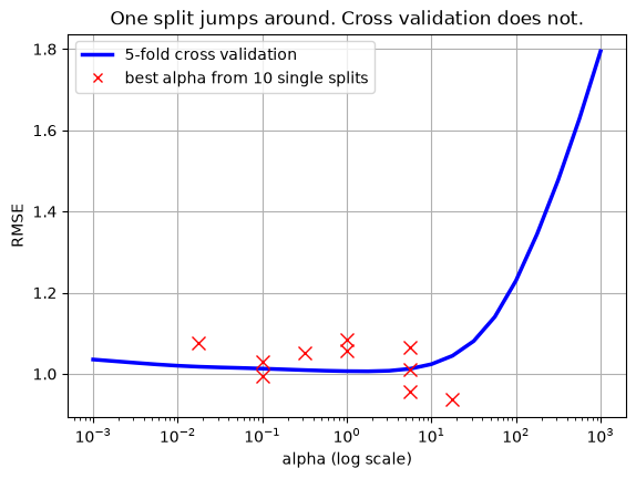
The blue curve is smooth and has a broad, shallow bottom. The red crosses are where ten single splits each thought the minimum was. They are scattered across three orders of magnitude, all sitting on a curve that is essentially flat underneath them.
Q4. Write this one out by hand
a. Why is the blue curve smoother than any one split’s curve would be?
b. The bottom of the blue curve is very flat, roughly from alpha 0.01 to alpha 10. What does that flatness tell you about how much the exact choice of alpha matters here?
c.GridSearchCV refits the model on all the data once it has chosen. Why is that the right thing to do, given that the whole point was to hold data out?
Leakage
This is a really important topic that you will see in the real world. One way to set yourself apart on the job market is to have a deep understanding of best practices when training models!!!
Leakage is when information from outside the training set gets into the training process. The model ends up knowing something it should not, so it scores well in testing and then falls apart in the real world. This is like cheating on a test by looking at the exam answers and then failing once you get a real job because you did not really learn the material. It is the single most common serious mistake in applied machine learning, and it is dangerous precisely because it does not look like a mistake. Nothing crashes. The number just comes out better.
We are going to build a dataset that contains no information whatsoever. 100 samples, 5000 features, every single number drawn at random. The labels are coin flips. There is nothing to learn. Any honest method must land at about 50 percent accuracy, because that is what guessing gets you.
Then we will do one very reasonable looking thing, and get 85 percent.
Q5. Write this one out by hand
The dataset below is pure noise, and the labels are coin flips.
Before you run it: we are going to pick the 20 features most correlated with the labels, out of 5000, and then cross validate a model using those 20. Do you expect that to score around 50 percent, or better than 50 percent?
Commit to an answer and a reason before you look.
Logistic Regression
In the code below we build a LogisticRegression model two ways! What is Logistic Regression?
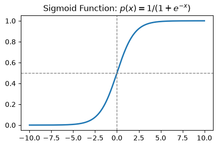
Even though it is called regression, Logistic Regression is a classification model (confusing right?). We basically adapt the Linear Regression model to be able to output yes/no answers by feeding the linear fit function into the sigmoid function:
This means it’s a linear model for the log-odds, not for p itself. We then use something like gradient descent to optimize the log-likelihood. Once the model is trained we would classify as 1 if p(x) > 0.5 and 0 otherwise (or whatever threshold we choose for the problem).
Trained two ways
BAD
In the bad version we use a feature selection tool called SelectKBest on all the data FIRST. This tool finds the best features using ANOVA F-value between feature and class labels. The output trims down our features to just the 20 “best” ones. Then we do our cross validation.
GOOD
In the good version we build a pipeline so that we do the SelectKBest only after the data has been split into folds, so we then apply that SelectKBest on the training portion of the data for that fold.
from sklearn.linear_model import LogisticRegressionfrom sklearn.feature_selection import SelectKBest, f_classifr = np.random.default_rng(seed=0)n_samples =100n_features =5000X_noise = r.standard_normal((n_samples, n_features)) # pure noisey_coin = r.integers(0, 2, n_samples) # coin flipsprint("There is no relationship at all between X_noise and y_coin.")print("Honest accuracy has to be about 0.50.\n")# ---- THE WRONG WAY ----# pick the 20 best features using ALL the data, then cross validate on those 20selector = SelectKBest(f_classif, k=20)selector.fit(X_noise, y_coin)X_selected = selector.transform(X_noise)wrong = cross_val_score(LogisticRegression(max_iter=5000), X_selected, y_coin, cv=5)print(f"WRONG, selecting features before cross validation. Score : {wrong.mean():.3f}")# ---- THE RIGHT WAY ----# put the selection INSIDE the pipeline, so it is redone from scratch on each# fold's training data and never sees the held out foldright_pipe = make_pipeline( SelectKBest(f_classif, k=20), LogisticRegression(max_iter=5000))right = cross_val_score(right_pipe, X_noise, y_coin, cv=5)print(f"RIGHT, selection happens inside each fold, Score : {right.mean():.3f}")
There is no relationship at all between X_noise and y_coin.
Honest accuracy has to be about 0.50.

WRONG, selecting features before cross validation. Score : 0.850
RIGHT, selection happens inside each fold, Score        : 0.480
0.850 against 0.480.
The leaky version got 37 points of extra accuracy out of data that contains nothing by cheating. If you had run only the first version, you would have reported a model that is 85 percent accurate at predicting a coin flip, and you would have believed it, because the code looks completely reasonable.
Here is what went wrong. When you search 5000 random features for the 20 that best match your labels, you will find 20 that match quite well, by chance. That matching is a property of these particular 100 labels, including the labels of the points that later end up in the held out part of the fold. So by the time cross validation runs, the features have already been chosen using the answers. The held out fold was never really held out.
The fix is the whole reason pipelines exist. Anything that learns something from the data has to happen inside the pipeline: scaling, feature selection, imputing missing values, encoding categories, oversampling. Then cross_val_score refits it from scratch on each fold’s training data, and the held out fold stays genuinely unseen.
The rule to remember
If a step looks at y, or computes any statistic from X (a mean, a standard deviation, a correlation, a category list), it learns. It belongs inside the pipeline.
The tell is .fit(). If a step has a .fit() method, putting it outside the pipeline is a leak waiting to happen.
Q6. Write this one out by hand
For each of these, say whether it leaks, and why.
a. You fill in missing values with the mean of the whole column, then split into train and test.
b. You split into train and test, then fill missing values in both using the mean of the training column.
c. You are predicting whether a customer will cancel next month. One of your features is “number of support calls in the last 90 days”, and it turns out that number was recorded after the cancellation.
d. You have 50 patients, each with 10 scans, so 500 rows. You split the 500 rows randomly into train and test.
e. You scale your features using the mean and standard deviation of the training set only, then apply that same scaler to the test set.
Stratification
There is another way for your test-train-validate split to lie to you, and this happens in data sets that are unbalanced or contain rare things. To apply stratification you need some form of categorical data, eg labels in classification tasks or a way to split up the data into bins for regression tasks.
Suppose 5 percent of your patients have the condition you are trying to detect. You have 200 patients, so 10 positives. Split that into 5 folds at random and each fold should get about 2 positives. Should!!!!
Stratification is where we guarantee a representative sample of our data population in each of our splits (or folds). There are a few places you might use this.
When you are creating your test-train split at the beginning. If you know that you have some rare observations in your labels you might stratify your test-train split on the y-labels:
from sklearn.model_selection import train_test_split

X_train, X_test, y_train, y_test = train_test_split(
    X, y,
    test_size=0.2,
    stratify=y,
    random_state=42
)
When you are doing cross validation. You want to tell your Kfold cross validation to stratify. Here we use the StratifiedKFold function to achieve this. When it is creating the folds it works to try to ensure there are representative samples of the rare data in each fold.
from sklearn.model_selection import KFold, StratifiedKFoldr = np.random.default_rng(seed=3)n =200X_rare = r.standard_normal((n, 4))y_rare = np.zeros(n, dtype=int)y_rare[:10] =1# only 10 positives out of 200X_rare[y_rare ==1] +=1.5# give the positives a real, learnable signalshuffle = r.permutation(n)X_rare, y_rare = X_rare[shuffle], y_rare[shuffle]print(f"{y_rare.sum()} positives out of {n}, so {y_rare.mean():.0%} of the data\n")plain = KFold(n_splits=5, shuffle=True, random_state=7)strat = StratifiedKFold(n_splits=5, shuffle=True, random_state=7)for label, splitter in [("KFold", plain), ("StratifiedKFold", strat)]: counts = []for train_idx, test_idx in splitter.split(X_rare, y_rare): counts.append(int(y_rare[test_idx].sum()))print(f" {label:16s} positives in each test fold: {counts}")
10 positives out of 200, so 5% of the data

  KFold            positives in each test fold: [3, 0, 3, 3, 1]
  StratifiedKFold  positives in each test fold: [2, 2, 2, 2, 2]
Think about what that means. In round 2, the model is tested on 40 patients, none of whom have the condition. You cannot measure how well it detects the condition, because there is nothing to detect in the data it was given. If you asked for accuracy you would get a lovely high score for a model that could be answering “no” to everything.
StratifiedKFold gives [2, 2, 2, 2, 2] every time. It splits each class separately, so every fold ends up with the same class balance as the full dataset.
Use StratifiedKFold for classification. Always. There is no cost and it removes a whole category of nonsense. Scikit-learn actually does this for you automatically when you pass an integer to cv= with a classifier, but be explicit, because when you build the splitter yourself the default is not stratified.
The same idea applies to your test set, which is what Geron’s Create a Test Set section is about. He splits California housing by income category rather than purely at random, so the test set has the same mix of income levels as the country. A test set that is not representative gives you an answer to the wrong question.
Q7. Write this one out by hand
a. In the fold with zero positives, a model that predicts “no condition” for every single patient scores 100 percent accuracy. Explain why that is worth being alarmed about, in a sentence a doctor would understand.
b. Stratification keeps the class balance the same in every fold. Name something other than the class label you might want to keep balanced across folds, and say why.
c. Is there any situation where you would deliberately not stratify? Have a think about it.
Nested Cross Validation
This is our last type of validation and maybe the most subtle.
We just used cross validation to choose alpha. Then we reported the cross validation score of the winner. Do you see the problem?
We tried 25 values and kept the best score. Some of that best score is real, and some of it is the luck of those particular folds. So the winner’s CV score is optimistic as an estimate of how the model does on new data, for exactly the reason the Day 3 validation score was.
Nested cross validation fixes it with two loops.
The inner loop does what we have been doing: split the training data into folds and pick the best hyperparameters.
The outer loop holds out a fold that the inner loop never saw at all, and scores the whole tuning procedure on it.
The outer score answers a different question. Not “how good is the model I picked”, but “how good is my whole process of picking a model”, which is the honest thing to report.
This is really confusing at first, so please go back and reread the last few sentences!
Below we run it on six small, noisy datasets, where 40 features hide only 2 that mean anything and a quarter of the labels are flipped on purpose.
We use the Logistic Regression model from earlier in these notes. Its hyperparameter is called C, and it does the same job alpha did for Ridge, just upside down: C is essentially 1/\alpha, so a smallC means heavy regularization. Six values of C on data this noisy is plenty of chances to get lucky.
from sklearn.datasets import make_classification# remember: small C means heavy regularization, it is like 1/alphaparam_grid = {"logisticregression__C": [0.001, 0.01, 0.1, 1, 10, 100]}not_nested = []nested = []for dataset inrange(6): X_hard, y_hard = make_classification( n_samples=80, n_features=40, n_informative=2, n_redundant=0, flip_y=0.25, random_state=dataset) base = make_pipeline(StandardScaler(), LogisticRegression(max_iter=5000))# inner loop: this is ordinary GridSearchCV, tuning on 5 folds search = GridSearchCV(base, param_grid, cv=KFold(5, shuffle=True, random_state=0), scoring="accuracy") search.fit(X_hard, y_hard)# outer loop: score the WHOLE search on folds it never tuned on.# cross_val_score refits `search` from scratch inside each outer fold. outer_score = cross_val_score( search, X_hard, y_hard, cv=KFold(5, shuffle=True, random_state=1)).mean() not_nested.append(search.best_score_) nested.append(outer_score)print(f" dataset {dataset}: not nested {search.best_score_:.4f} "f"nested {outer_score:.4f} difference {search.best_score_-outer_score:+.4f}")gaps = np.array(not_nested) - np.array(nested)print(f"\nmean optimism = {gaps.mean():+.4f}")print(f"positive on {int((gaps>0).sum())} of 6 datasets")
  dataset 0:  not nested 0.6500   nested 0.5250   difference +0.1250
  dataset 1:  not nested 0.6000   nested 0.4750   difference +0.1250
  dataset 2:  not nested 0.6625   nested 0.5875   difference +0.0750
  dataset 3:  not nested 0.8875   nested 0.8375   difference +0.0500
  dataset 4:  not nested 0.7375   nested 0.7125   difference +0.0250
  dataset 5:  not nested 0.5750   nested 0.5875   difference -0.0125

mean optimism = +0.0646
positive on 5 of 6 datasets
On dataset 0 the not nested model reports 0.6500 accuracy and the nested estimate is 0.5250. On dataset 1 it is 0.6000 against 0.4750, which is below chance aka flipping a coin has higher accuracy. The tuning found patterns in the noise, congratulated itself, and the nested loop caught it.
Across all six the mean optimism is +0.0646, and it is positive on 5 of 6. That last detail matters: it is not positive every single time, and on dataset 5 it actually comes out slightly negative, at -0.0125, because these are small noisy datasets and everything wobbles. But it leans one direction, and that direction is always giving yourself more credit than you deserve!
When does this matter? When your dataset is small, your hyperparameter grid is large, or your signal is weak. Any of those, and you should nest. With thousands of clean samples and three values of alpha, the effect is tiny and not worth the compute. Cross validation costs you k fits, and nesting costs you k times as many again.
The version we will actually use
Nested cross validation is the careful answer, and most of the time it is more machinery than you need. Here is the version people actually use in the real world, and the reason it works.
Look again at what the outer loop is doing. It holds out a chunk of data, runs the entire tuning procedure on everything else, and then scores the result on the chunk it held out. That is exactly what a test set is. Nested cross validation is just doing that five times and averaging.
So you can do the same thing once:
Split off a test set at the very start, and do not touch it.
Tune however you like on everything else, with cross validation, trying as many values as you want.
Score the finished model on the test set. Once.
Step 3 is an outer fold. Your tuning never saw that data, so the number is honest for exactly the same reason the nested score was honest.
What you give up is precision, not honesty. Nested cross validation averages five outer scores, so there is less chance that it is randomly a little high or a little low. One test set gives you one number based on one slice of data, so it could have more variation (high/low). Both are unbiased, one is just measured more carefully.
We really only use Nested Cross Validation in special cases where it is high impact: small data sets, lots of hyperparameters, or a very weak signal. Most of the time just honestly holding out a test set to use at the very end is enough! We accept a small chance of variation that comes with basically the same honesty for much less compute time. And compute time is a real limited resource!
So, for the rest of the semester we will split off a test set first, and then do all of our tuning, cross validation, statistics, etc by looking only at the training data (split into training and validation folds)
Q8. Write this one out by hand
a. In your own words, what question does the nested score answer that the non-nested score does not?
b. Dataset 1 came out at 0.4750 nested, which is worse than guessing. What should you actually do with that model?
c. The mean optimism was +0.0646, but on dataset 5 it came out negative, at -0.0125, meaning the nested score was slightly better than the non-nested one. Does that mean nesting was pointless there? What would you have known in advance?
d. Nesting 5 outer folds around 5 inner folds with 6 values of C means fitting the model 150 times. Given that, when would you skip nesting and just hold out a test set instead?
Putting It Together
The workflow for the rest of this course, and for your final project:
Split off a test set first, before you explore anything. Stratify it if you are classifying. Then leave it alone.
Build a pipeline with every step that learns anything inside it.
Tune with GridSearchCV on the training data, using StratifiedKFold for classification.
Look at the spread across folds, not just the mean.
Once, at the very end, score the finished model on the test set. That is the number you report.
If the test score is disappointing and you go back and change things, be honest with yourself that your test set is now partly used up.
You Try: optional code
Nothing here is collected. Work through it if you want the idea to stick.
1. In the leakage example, change k=20 to k=2 and then to k=200. Does selecting fewer features make the leak smaller or bigger? Guess first, then explain what you got.
2. Change the leakage example from 5000 features to 50. How much of the fake accuracy survives? What does that tell you about which datasets are most dangerous?
3. In the stratification example, change random_state=7 to a few other numbers and watch the KFold counts move around while the StratifiedKFold counts never do.
4. Take the Day 3 alpha sweep and redo it with RidgeCV, which does cross validation internally:
from sklearn.linear_model import RidgeCV
model = make_pipeline(
    PolynomialFeatures(degree=15, include_bias=False),
    StandardScaler(),
    RidgeCV(alphas=alphas))
model.fit(X, y)
print(model[-1].alpha_)
Does it agree with what GridSearchCV chose?
Before Next Class
In your lecture notes notebook, add your hand written notes and answers to the questions.
Finish the Day 4 practice problems in HW_day4.ipynb, and Weekly Homework 2, due Sunday 9/13 at 11:59pm, which covers Day 3 and Day 4.
Read Geron chapter 3, the section on Performance Measures.
Watch the Day 5 video on the class website.
Today was about trusting your numbers. Day 5 is about the fact that one number was never enough in the first place. We saw a preview of it here: a model that says “no condition” to every patient scored 100 percent on a fold with no positives. Accuracy can hide almost anything, and next class we look at what to use instead.
Answers to the Q Boxes
Try every one of these by hand first. These are short summaries, not full answers, and the writing out is the part that does the work.
Q1. Three sets
a. The validation set is for making choices, and you can look at it as many times as you like. The test set is for estimating performance on new data, and you look at it once.
b. No. You picked the winner out of 200 partly because it got lucky on that validation set, so its validation score includes that luck. The more things you try, the more optimistic that number gets.
c. You are the leak. If you explore everything first you will notice patterns, and every choice you make afterwards is shaped by things you saw in the test set, even though no code ever touched it.
Q2. Guess the spread
The chosen alpha ranged from 0.018 to 17.783, a factor of about 1000. Most people guess a factor of 2 or 3. Being surprised here is the point of the exercise.
Q3. Reading k-fold
a. 160 points to train on, 40 to test on, each round.
b. Five times, once per fold.
c. Advantage: almost all your data is used for training every time, which is valuable when you have very little of it. Disadvantages: you fit the model 200 times, which is slow, and each individual test is a single point, so the scores are extremely noisy even though the average is fine.
d. Something like “on held out data this model is typically off by about 1.0, and depending on which slice we test it ranges from about 0.86 to 1.09.” Give the range, not just the mean.
Q4. Reading the comparison plot
a. Each point on the blue curve is the average of five separate held out scores, so a lot of the fold-to-fold noise cancels out. One split has no averaging at all.
b. It tells you the exact choice barely matters. Anything from about 0.01 to 10 gives essentially the same performance, so agonizing over the third decimal place of alpha is wasted effort.
c. Cross validation was for choosing, and it is finished once the choice is made. Now you want the best possible model, and more training data makes a better model. Holding data out permanently would just waste it.
Q5. Predicting the leak
It scores far better than 50 percent, about 85 percent. If you guessed 50 you were reasoning correctly about the data and had not yet met this trap, which is exactly why the example is here.
Q6. Leak or not
a.Leaks. The mean was computed using the test rows, so information about them is baked into the training data.
b.Fine. The statistic came from the training set only, which is the correct order.
c.Leaks, and this is the nastiest kind. The feature is recorded after the thing you are predicting, so it could not possibly be available when you actually need a prediction. This is called a time leak and it is very common in real projects.
d.Leaks. The same patient appears in both train and test. The model can recognize the patient rather than the condition. You have to split by patient, not by row. Look up GroupKFold.
e.Fine. This is exactly the right way to do it.
Q7. Stratification
a. A model that says “nobody has it” is useless and would score perfectly on that fold. So a high accuracy on a rare condition tells a doctor nothing about whether the model can actually find the sick patients.
b. Reasonable answers: time period, so every fold has a mix of old and new data. Site or hospital, so one location does not dominate. Any demographic group you care about performing evenly across. The general idea is anything whose imbalance across folds would make the folds not comparable.
c. Yes, when the ordering carries meaning. Time series is the main one: with data over time you want to train on the past and test on the future, so you use TimeSeriesSplit and deliberately do not shuffle or stratify. Shuffling would let the model train on next week and test on last week.
Q8. Nested cross validation
a. The non-nested score says how good the chosen model looked on the folds used to choose it. The nested score says how good the whole procedure of choosing is, measured on data that had no part in the choosing.
b. Nothing. Do not deploy it. Below chance on held out data means it learned noise, and the honest report is that this data does not support a model.
c. Not pointless. You only know the optimism was near zero because you nested. Without it you had no way to tell dataset 5 from dataset 1, where the same procedure was inflated by 0.125. A small negative number is not “nesting was wrong”, it is just noise on 80 points, and it is worth expecting rather than being surprised by.
d. When the fits are expensive, or the dataset is big enough that a held out test set is still large. With plenty of data, splitting off a test set once gives you an honest number for the price of one extra fit rather than 150.