Classification Metrics
What each one tells you, and what it cannot
How to use this sheet
This is the reference for Day 5. It is not a lecture, it is the thing you open when you are writing a report and cannot remember whether precision is the row or the column. Every metric gets the same four things: what it is, what it tells you, what it cannot tell you, and how to get it in sklearn.
Two things to keep straight the whole way through:
y_predis 0 or 1 for each sample. It comes frommodel.predict(X), and it depends on a threshold (0.5 by default).y_probis a probability for each sample. It comes frommodel.predict_proba(X)[:, 1], and it does not depend on any threshold.
Half the metrics below take one and half take the other, and passing the wrong one is the most common mistake in this whole topic. Some functions error when you do it. roc_auc_score does not, it just gives you a wrong number.
Which data do you compute these on? The validation set, or out-of-fold predictions from cross_val_predict on the training data. Every number on this sheet is a number you look at while you are still making choices (which threshold, which model), and choices get made on validation data. The test set is opened once, at the very end, after every choice is made, and the numbers you compute there go in the report and do not get revisited. If you find yourself picking a threshold by watching a test set score go up, you no longer have a test set.
The positive class is 1. Everything below, “positive” means the thing you are trying to find: the good wine, the malignant tumor, the fraud. If your data stores that as 0, flip it before you do anything else (the Day 5 homework has an example).
The confusion matrix
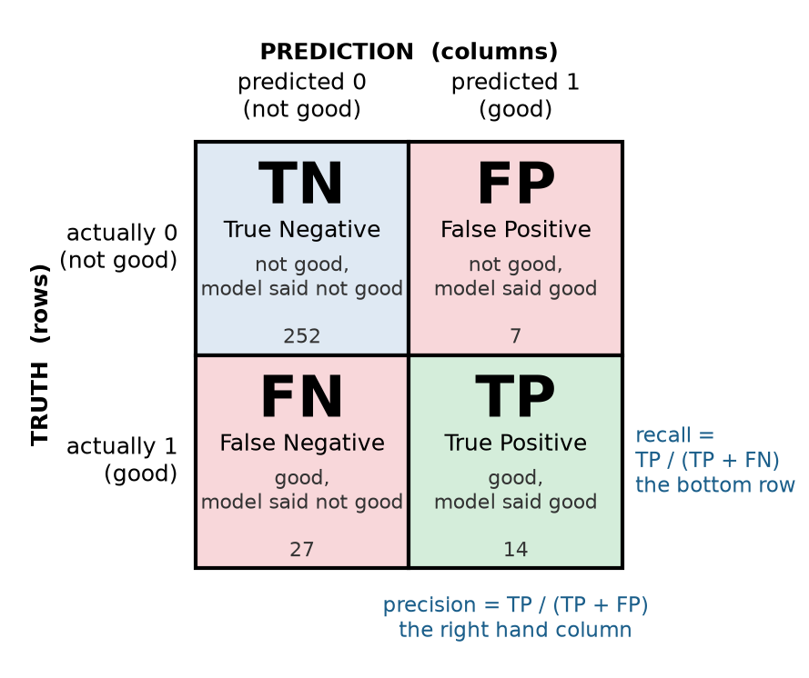
What it is. A 2 by 2 table of counts. Rows are the truth, columns are the prediction, and class 0 comes first.
| predicted 0 | predicted 1 | |
|---|---|---|
| actually 0 | TN | FP |
| actually 1 | FN | TP |
- TN, true negative. It is not the thing, and the model said it is not. Usually most of the data.
- FP, false positive. It is not the thing, but the model said it is. A false alarm.
- FN, false negative. It is the thing, and the model missed it.
- TP, true positive. It is the thing, and the model caught it.
What it tells you. Everything. Every other number on this sheet is computed from these four cells, so if you have the matrix you can work out all of them by hand. It also tells you which kind of mistake the model makes, which no single number can.
What it cannot tell you. It is for one threshold. Change the threshold and you get a different matrix. It also does not scale to “is this model better than that one” very well, because you have four numbers to compare instead of one.
from sklearn.metrics import confusion_matrix
cm = confusion_matrix(y_true, y_pred)      # takes y_pred (0/1), not y_prob
tn, fp, fn, tp = cm.ravel()                # the four cells, in this order
Accuracy
What it is. The share of predictions that were right.
\text{accuracy} = \frac{TP + TN}{TP + TN + FP + FN}
What it tells you. How often the model is right, overall, at this threshold. Fine when the classes are balanced and both kinds of mistake cost about the same.
What it cannot tell you. Anything useful when one class is rare. If 3 percent of cases are positive, a model that says “no” every time is 97 percent accurate and has never found anything. Accuracy also cannot tell you which kind of mistake you are making.
Always compare it to the baseline. The baseline is the accuracy of a model that always predicts the majority class, which is just the share of the majority class. If your accuracy is not clearly above that, the model has not done anything.
from sklearn.metrics import accuracy_score
accuracy_score(y_true, y_pred)             # takes y_pred
baseline = 1 - y_true.mean()               # accuracy of "always predict 0", when 1 is the rare class
Precision
What it is. Of everything the model called positive, the share that really was.
\text{precision} = \frac{TP}{TP + FP}
It lives in the positive prediction column of the confusion matrix.
What it tells you. How much to trust a yes. Precision 0.67 means that when the model says “good wine,” it is right about two thirds of the time. Put it first when a false positive is the expensive mistake: spam filters, recommendations, anything that acts on a yes automatically, anything where a wrong yes lands on a real person.
What it cannot tell you. How many of the real positives you found. A model can have perfect precision by saying yes exactly once, to the one case it is surest about, and missing everything else. Precision on its own is also undefined for a model that never says yes (0 over 0), which sklearn reports as 0 with a warning.
from sklearn.metrics import precision_score
precision_score(y_true, y_pred)            # takes y_pred
Recall
What it is. Of everything that really was positive, the share the model found. Also called sensitivity and the true positive rate, and all three names mean exactly this.
\text{recall} = \frac{TP}{TP + FN}
It lives in the actually positive row of the confusion matrix.
What it tells you. How much of the thing you are looking for you actually caught. Recall 0.34 means you found 34 percent of the good wines and missed the rest. Put it first when a false negative is the expensive mistake: disease screening, fraud, defect recalls, anything where missing one is a disaster.
What it cannot tell you. How many false alarms you raised to get there. A model that says yes to everything has recall 1.0 and is useless. Recall is exactly zero for a model that never says yes, which is the number that exposes the “always no” model that accuracy hides.
from sklearn.metrics import recall_score
recall_score(y_true, y_pred)               # takes y_pred
Precision and recall together, and the threshold
Precision and recall pull against each other, and the thing that moves them is the threshold.
predict() says 1 when y_prob is at least 0.5. That 0.5 is a default, and you can pick your own:
y_prob = model.predict_proba(X)[:, 1]
y_pred_custom = (y_prob >= 0.3).astype(int) # your threshold, your predictions- Lower the threshold: more yeses, so recall goes up and precision goes down.
- Raise the threshold: fewer yeses, so precision goes up and recall goes down.
There is no threshold that makes both high, unless the model separates the classes perfectly. The threshold is a decision about which mistake you would rather make, and it belongs to whoever uses the model, not to sklearn.
precision_recall_curve computes precision and recall at every possible threshold at once:
from sklearn.metrics import precision_recall_curve
precisions, recalls, cutoffs = precision_recall_curve(y_true, y_prob)   # takes y_prob
# precisions and recalls are one entry longer than cutoffs
F1 score
What it is. One number that combines precision and recall. It is the harmonic mean, which gets dragged toward whichever of the two is smaller, so you cannot get a high F1 by being great at one and terrible at the other.
F_1 = 2 \cdot \frac{\text{precision} \cdot \text{recall}}{\text{precision} + \text{recall}}
What it tells you. A single score for comparing models when you have no reason to care more about one kind of mistake than the other. Handy for a leaderboard.
What it cannot tell you. Which mistake you are making. Two models with the same F1 can be opposite: one high precision and low recall, the other the reverse. F1 also weights the two equally, which is almost never what the actual problem wants. Never let it be the only number in a report.
from sklearn.metrics import f1_score
f1_score(y_true, y_pred)                   # takes y_pred
False positive rate
What it is. Of everything that really was negative, the share the model wrongly called positive.
\text{FPR} = \frac{FP}{FP + TN}
What it tells you. How often a negative case gets a false alarm. It is the x axis of the ROC curve. (Its opposite, 1 - \text{FPR}, is called specificity, and you will hear that word in medical settings.)
What it cannot tell you. How bad the false alarms are relative to the positives. The denominator is the number of negatives, so when negatives are most of the data, a lot of false positives still makes a small rate. 7 false alarms out of 259 negatives is 2.7 percent, and looks tiny, even when those same 7 are a third of everything the model called positive.
The ROC curve and ROC AUC
What it is. The ROC curve plots recall (true positive rate) against the false positive rate, one point for every threshold. AUC is the area under it: 1.0 is a perfect ranking, 0.5 is random guessing.
What it tells you. How well the model ranks positives above negatives, across all thresholds at once. AUC 0.87 means: pick a random positive and a random negative, and the model gives the positive the higher probability 87 percent of the time. It is the standard number for comparing two models, and the one you will see most in papers and interviews.
What it cannot tell you.
- What happens at any particular threshold. AUC never looks at
y_pred, so it says nothing about how many cases you will miss or flag once you deploy. - Anything honest when positives are rare. Because the FPR denominator is the number of negatives, the ROC curve flatters a model on imbalanced data. The same model that has AUC 0.87 on the wine data has average precision 0.53.
- It is not an accuracy. “AUC 0.95 so it is 95 percent accurate” is wrong.
from sklearn.metrics import roc_curve, roc_auc_score
fpr, tpr, cutoffs = roc_curve(y_true, y_prob)     # takes y_prob
roc_auc_score(y_true, y_prob)                     # takes y_prob. Passing y_pred runs, and is wrong.
The precision/recall curve and average precision
What it is. The PR curve plots precision against recall, one point for every threshold. Average precision (AP) is roughly the area under it. Random guessing sits at a flat line at the share of positives, not at 0.5.
What it tells you. The same trade off as the ROC curve, but measured against the positives instead of the negatives, so it stays honest when positives are rare. A low AP with a high AUC is the signature of an imbalanced dataset: the model ranks well, but you cannot get high recall without accepting a lot of wrong yeses.
What it cannot tell you. Again, nothing about one specific threshold. And AP is less widely recognized than AUC, so when you report it, say why you chose it.
Which one to report. Positives rare and you care about the positives: PR and AP. Classes balanced or you care about both kinds of error equally: ROC AUC. Not sure: show both and say why they disagree.
from sklearn.metrics import precision_recall_curve, average_precision_score
precisions, recalls, cutoffs = precision_recall_curve(y_true, y_prob)   # takes y_prob
average_precision_score(y_true, y_prob)                                 # takes y_prob
Calibration
What it is. Whether the probabilities mean what they say. A model is calibrated if, among all the cases it gave about 0.7 to, about 70 percent really are positive. The calibration curve plots the real share of positives against the average predicted probability, in bins, and a calibrated model sits on the diagonal.
What it tells you. Whether you can use y_prob as an actual probability. This matters the moment a person acts on the number itself: “70 percent chance this is malignant” is a sentence a doctor makes decisions with.
What it cannot tell you. Whether the model ranks well. A model can rank perfectly (AUC 1.0) and be terribly calibrated, for example by giving every positive 0.51 and every negative 0.49. Calibration and AUC are separate questions. Also, bins with few samples in them tell you very little: a bin of 8 wines cannot say whether the model is overconfident.
Get the probabilities honestly. Probabilities from predict_proba on the training data are overconfident, because the model already saw those answers. Use cross_val_predict, so each prediction comes from a model that did not train on that row. Put the scaler inside a pipeline for the Day 4 reason.
from sklearn.model_selection import cross_val_predict
from sklearn.calibration import calibration_curve
y_prob_cv = cross_val_predict(pipe, X_train, y_train, cv=5, method="predict_proba")[:, 1]
true_share, predicted_avg = calibration_curve(y_train, y_prob_cv, n_bins=5)
# note the order: the real share comes back first, the predicted average second
Logistic regression is usually reasonably calibrated. Random forests and support vector machines often are not, and CalibratedClassifierCV exists to fix them.
Which number, in one table
| You want to know… | Look at | Needs |
|---|---|---|
| is the model doing anything at all | accuracy against the always-majority baseline | y_pred |
| which kind of mistake it makes | confusion matrix | y_pred |
| can I trust a yes | precision | y_pred |
| did it find the real ones | recall | y_pred |
| one number to compare models, mistakes cost the same | F1 | y_pred |
| which of two models ranks better, balanced classes | ROC AUC | y_prob |
| which of two models ranks better, rare positives | average precision | y_prob |
| what happens at the threshold I will deploy | confusion matrix at that threshold | y_prob and a threshold |
| does 0.7 mean 70 percent | calibration curve | y_prob, from cross_val_predict |
And the one sentence every report needs: which mistake is more expensive for this problem, and therefore whether you tuned for precision or for recall.