# We will just go ahead and import all the useful packages first.
import numpy as np
import sympy as sp
import pandas as pd
import matplotlib.pyplot as plt

# Special Functions
from sklearn.metrics import r2_score, mean_squared_error

# Functions to deal with dates
import datetimeMath for Data Science
Calculus - Optimization
Important Information
- Email: joanna_bieri@redlands.edu
- Office Hours take place in Duke 209 unless otherwise noted – Office Hours Schedule
Today’s Goals:
- Use our understanding of derivatives for optimization
- Review - First derivative test
- Second Derivative
- Optimization example
Derivative Definition
\[ \frac{dy}{dx} = \lim_{dx\to 0} \frac{f(x+dx) - f(x)}{dx} \]
First Derivative Test
- The function has a local maximum or minimum whenever the derivative equals zero:
\[\frac{dy}{dx}=0\]
we solve this for all of the x-values where this is true, \(x^*\).
- The points \((x^*,y(x^*))\) where the derivative equations zero are called “stationary points” or “critical points”
- We can tell if a critical point is a local max by the derivative going from increasing to decreasing, positive to negative, as we cross the point.
- We can tell if a critical point is a local min by the derivative going from decreasing to increasing, negative to positive, as we cross the point.
Global Maximum and Minimum
Check y-values of all of the critical points but also check the end points or take the limit if there are no clear endpoints.
# Get the data and functions from last time

file_location = 'https://joannabieri.com/mathdatascience/data/NationalPark.csv'
DF = pd.read_csv(file_location)

# Data Representation of our function
xreal = DF['Day']
yreal = DF['Visitors']
yfit = -4.80852601194688e-10*xreal**5 + 4.82804864082977e-7*xreal**4 - 0.000164214937971268*xreal**3 + 0.0211869075069019*xreal**2 - 0.789424620226024*xreal + 106.945375713063
yfit_p = -2.40426300597344e-9*xreal**4 + 1.93121945633191e-6*xreal**3 - 0.000492644813913804*xreal**2 + 0.0423738150138038*xreal - 0.789424620226024

# Symbolic Representation of our function
x = sp.symbols('x')
y = -4.80852601194688e-10*x**5 + 4.82804864082977e-7*x**4 - 0.000164214937971268*x**3 + 0.0211869075069019*x**2 - 0.789424620226024*x + 106.945375713063
y_p = sp.diff(y,x)
Can we take the derivative of the derivative?
Questions
- What does the derivative tell us?
- What does it mean to take the derivative of the derivative?
- What is the rate of change of the rate of change?
Look at the graph of \(y=f(x)\)
plt.plot(xreal,yreal,'k.')
plt.plot(xreal,yfit,'b-')
plt.grid()
plt.xlabel('Day of Year')
plt.ylabel('Number of Visitors')
plt.show()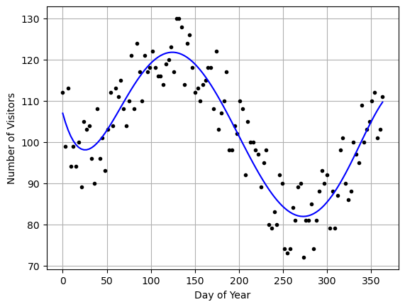
#from IPython.display import Video

# Animation code created by Google Gemini AI
# Altered by Joanna
# Let me know if you want to see this code!

#Video("Tangent.mp4")
If the derivative tells us about the change in the function or the slope… what does the change in the derivative tell us?
The second derivative tells us the change in slope
What does a changing slope mean?
- If the slope does not change - then we have a straight line
- If the slope changes by getting more positive - then we have a function that is curving upwards
- If the slope changes by getting more negative - then we have a function that is curving downward
The second derivative tells us about the curvature of the function
The notation for the second derivative:
\[\frac{d^2y}{dx^2}\]
This tells us how curved our function is at different points.
In terms of this application “how quickly is my decrease in visitors changing to an increase in visitors” OR “How fast are we going from increasing to decreasing”
SYMPY can do the second derivative
# Find the symbolic derivative

y_pp = sp.diff(y,x,x)
print(y_pp)
-9.61705202389376e-9*x**3 + 5.79365836899572e-6*x**2 - 0.000985289627827608*x + 0.0423738150138038# Get the Data Representation
yfit_pp = -9.61705202389376e-9*xreal**3 + 5.79365836899572e-6*xreal**2 - 0.000985289627827608*xreal + 0.0423738150138038
plt.plot(xreal,yfit_pp,'g')
plt.grid()
plt.xlabel('Day of Year')
plt.ylabel('Change in the Rate of Change of Visitors')
plt.show()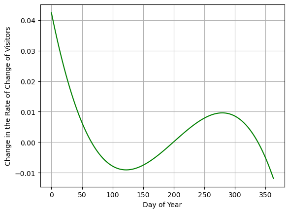
What does this tell me?
- Where is our function the most curvy?
- Where is our function curved upward?
- Where is our function curved downward?
- Where does our function act kinda like a straight line - zero curvature?
Do our answers here make sense?
# This code is way more advanced that you need to know how to do
# I want to show these graphs side by side

fig, (ax1, ax2, ax3) = plt.subplots(1, 3, figsize=(14, 5))

ax1.plot(xreal,yfit,'b',label = 'y=f(x)')
ax1.grid()
ax1.set_xlabel('Day of Year')
ax1.set_ylabel('f(x)')
ax1.axhline(y=0, color='black', linestyle='--', linewidth=2)
# Add the max min points
R = list(sp.roots(y_p))
ax1.plot(R[0],y.subs(x,R[0]),'or')
ax1.plot(R[1],y.subs(x,R[1]),'or')
ax1.plot(R[2],y.subs(x,R[2]),'or')


ax2.plot(xreal,yfit_p,'m',label = "y'=df/dx")
ax2.grid()
ax2.set_xlabel('Day of Year')
ax2.set_ylabel('First Derivative')
ax2.axhline(y=0, color='black', linestyle='--', linewidth=2)
ax2.plot(R[0],y_p.subs(x,R[0]),'or')
ax2.plot(R[1],y_p.subs(x,R[1]),'or')
ax2.plot(R[2],y_p.subs(x,R[2]),'or')

ax3.plot(xreal,yfit_pp,'g',label = "y''=d2f/dx2")
ax3.grid()
ax3.set_xlabel('Day of Year')
ax3.set_ylabel('Second Derivative')
ax3.axhline(y=0, color='black', linestyle='--', linewidth=2)
ax3.plot(R[0],y_pp.subs(x,R[0]),'or')
ax3.plot(R[1],y_pp.subs(x,R[1]),'or')
ax3.plot(R[2],y_pp.subs(x,R[2]),'or')

plt.tight_layout()
plt.show()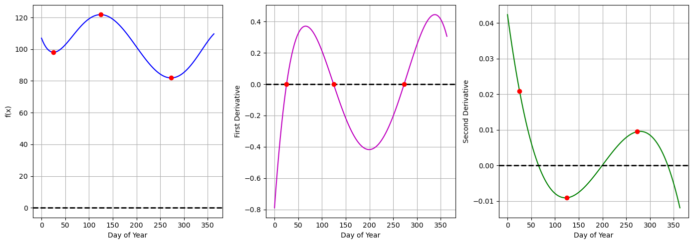
Can the second derivative say anything about Critical Points?
The red dots in the plots represent the location of the critical points \(x^*\) and the values on each of the curves. So notice that in the original function (blue) these red dots are at the maximum and minimum points. On the derivative function (green) these points are all when the derivative is zero. What do you notice about these points on the second derivative function (green)?
- If my critical point \(x^*\) is a minimum then my second derivative is ___________. (and vice versa)
- If my critical point \(x^*\) is a maximum then my second derivative is ___________. (and vice versa)
This is called the second derivative test
You can use either the first or second derivative test to figure out whether a critical point that you found is a maximum or minimum.
Optimization
Optimization means finding maximums and minimums of some function. There are lots of situations where you might want to maximize or minimize something:
- Economics (Thanks Mia!) - we often want to minimize the cost of production - but this cost depends on the price of various components in the development of the product, the cost of labor (number of employees), and possible the capital cost (debt or rent).
- Medicine - we often have some idea of how a drug is absorbed or eliminated and we want to make sure the maximum or minimum dose remains below/above some safe/effective amount.
- Video Games - so many video games are based on optimization - League of Legends: Effective health when defending against physics damage is a function of Armor and Health - which can be purchased. How can you best spend your money?
Economics Example
Say you own a company and and you have been tracking the cost to manufacture your product. The product is made up of the following items
4 propellers that cost 2 dollars each
1 drone body that costs 8 dollars
2 HD cameras that cost 15 dollars each
TOTAL = \(46x\)
When we buy more product we can start to negotiate a better price: \(-0.6 x^2\)
To keep our office open it costs us 1000 per month: \(1000\)
If we buy too much material it actually starts to cost us money because of storage for the materials and inefficiency in organizing that much stuff: \(0.01 x^3\)
When we add all these ideas together we get a TOTAL cost function:
\[C(x) = 0.01 x^3 - 0.6 x^2 + 46 x + 1000 \]
How can we minimize the cost per drone, so that we are getting the biggest return on our work?
Plot the Cost Function
def C(x):
    return 0.01*x**3 - 0.6*x**2+46*x+1000

xdata = np.arange(1,200)
yc = C(xdata)

plt.plot(xdata,yc)
plt.grid()
plt.show()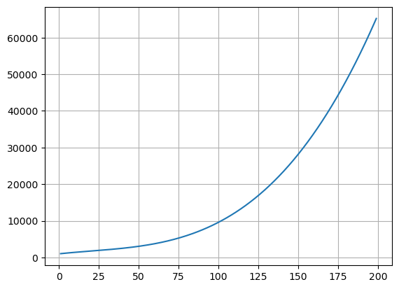
So this makes sense - as we increase the number of drones we make our cost keeps increasing. But is this how we get the most profit, just keep making more? Is the cost always increasing at the same rate?
We want to make sure that we make our drones for as little as possible and then sell them for as much as possible. Let’s say that the market price for one of our drones is $200.00. Then we need to know the cost of one of our drones to figure out the profit!
\[Profit = Revenue - Cost = 200 - Cost\]
So we want to minimize the cost per drone!
Find the Average Cost per Drone
If \(x\) represents number of drones then dividing by \(x\) will give us cost per drone.
\[A(x) = \frac{C(x)}{x} = 0.01 x^2 - 0.6 x + 46 + \frac{1000}{x}\]
Plot the Average Cost per drone
def A(x):
    return 0.01*x**2 - 0.6*x+46+1000/x

ya = A(xdata)

plt.plot(xdata,ya)
plt.grid()
plt.show()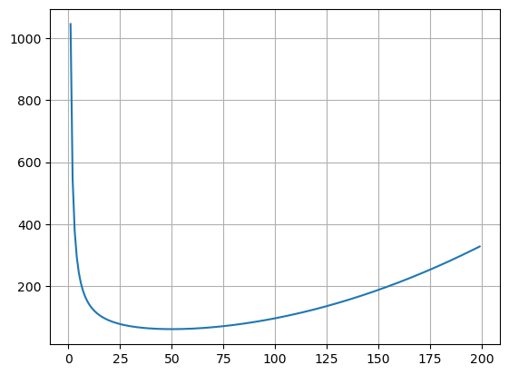
Let’s use Derivatives to Minimize!
- Find the critical point(s)
- Decide if the represent local max or min
- Decide if they represent global max or min
- Interpret the results
# Symbolic Function
x = sp.symbols('x',real=True,positive=True)
y = A(x)
y
\(\displaystyle 0.01 x^{2} - 0.6 x + 46 + \frac{1000}{x}\)
# Take the Derivative
y_p = sp.diff(y)
y_p
\(\displaystyle 0.02 x - 0.6 - \frac{1000}{x^{2}}\)
# Multiply by x^2 - to get rid of discontinuity x is never zero.
# Then find the roots t0 see where the derivative is zero
sp.roots(x**2*y_p)
{50.0000000000000: 1, -10.0 - 30.0*I: 1, -10.0 + 30.0*I: 1}# Check that 50 is a root of the derivative
y_p.subs(x,50)\(\displaystyle 0\)
# Lets do the first derivative test
xL = 49
xR = 51
print(y_p.subs(x,xL))
print(y_p.subs(x,xR))
-0.0364931278633902
0.0355324875048059# Lets do the second derivative test
y_pp = sp.diff(y,x,x)
y_pp.subs(x,50)\(\displaystyle 0.036\)
Is this the global minimum?
What do all these calculations tell us?
Well we only have one real critical point at \(x=50\). We could graph the derivative function if we wanted to check this.
This critical point is a minimum:
- First Derivative Test: The slope goes from negative to positive so we are in a valley
- Second Derivative Test: The function is curved up so our point is in a valley.
So we can interpret this result as - we will have minimum cost per drone if we make \(50\) of them. This cost per drone is…
A(50)61.0\(61\) dollars. So our profit per drone at this point is \(P = 200-61 = 139\). We make \(139\) dollars per drone. Or a total profit per month of \(139*50 = 6950\).
Is this a global minimum for \(A\)? Look back at the graph and think about the limits:
\[ \lim_{x\to0}0.01 x^2 - 0.6 x + 46 + \frac{1000}{x}\]
\[ \lim_{x\to\infty}0.01 x^2 - 0.6 x + 46 + \frac{1000}{x}\]
These limits both go to infintiy, so we have found a global minimum for the cost per drone at \((50,61)\).
Now we could make more drones to generate more profit overall, but we are not getting the most profit out of every drone we make anymore.
Here is a plot of the profit per drone
def price_per_drone(d,price=200):
    return (price-A(d))

d = np.arange(1,150,1)
prof = price_per_drone(d)

plt.plot(d,prof)
plt.axhline(y=0, color='black', linestyle='--', linewidth=2)
plt.axvline(x=50, color='black', linestyle='--', linewidth=2)
plt.grid()
plt.xlabel('number of drones')
plt.ylabel('price per drone')
plt.show()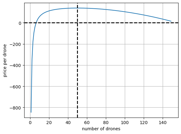
You try - Drug Absorption Example
Idea from: https://matheducators.stackexchange.com/questions/1550/optimization-problems-that-todays-students-might-actually-encounter
The concentration of caffeine \(C\) in the body at time \(t\) is modeled by the function:
\[c(t)=\frac{D}{1-\frac{\beta}{\alpha}}\left(e^{-\beta t}- e^{-\alpha t}\right)\]
here \(\alpha\) is the absorption rate and \(\beta\) is the elimination rate. \(D\) is the dose measured in mg. Parameters vary per person but entered below are the ones we will use:
\[\alpha = 0.33\] \[\beta = 0.33/60\] \[ D = 95 \]
Graph the function
# Absorption rate (per min)
a = .33
# Elimination rate (per min) 0.09 and 0.33 (per hour)
b = .33/60
# Dose - 1 cup ~ 95 mg
D = 95

def c(t):
    return D/(1-b/a)*(np.exp(-b*t)-np.exp(-a*t))

num_hours = 4
t = np.arange(0,num_hours*60,1)
caf = c(t)

plt.plot(t,caf)
plt.grid()
plt.xlabel('time since dose')
plt.ylabel('caffeine in body')
plt.show()
Questions:
- Assuming you drink one cup of coffee at 9am in the morning. When will you have the maximum amount of caffeine in your system? How much is in your system at that time?
- Does changing the dose change the time at which you will reach your maximum concentration? Redo the analysis for D=200, D=500, and D=0. Explain the results.
- Now that you know the time at which this function reaches a maximum (for the given \(\alpha\) and \(\beta\) values), calculate a minimum safe dose of caffeine. Let’s say you have a patient who can only have 25mg of caffeine in their system at one time, how big can their dose be? (HINT, Solve for D by hand, plug in your \(t^*\) and let \(c(t^*)=25\))
Make sure to graph the function, the derivative, and the second derivative.
You Try - Video Game Example
Idea from: https://matheducators.stackexchange.com/questions/1550/optimization-problems-that-todays-students-might-actually-encounter
In the video game League of Legends, a player’s Effective Health when defending against physical damage is given by
\[ E=\frac{H(100+A)}{100} \]
where \(H\) is health and \(A\) is armor. Health costs 2.5 gold per unit, and Armor costs 18 gold per unit. This is a bit more tricky because we have a function of two variables here. To find a single maximum we need another constraint. Usually in games you are constrained by the amount of gold you have. This is what we will do.
Questions
Imagine that you have 3600 gold, and you need to optimize the effectiveness E of your health and armor to survive as long as possible against the enemy team’s attacks. How much of each should you buy?
- First, consider that you can spend your money as \[ 3600 = 2.5H + 18A \] since you have 3600 gold and armor and health cost 2.5 and 18 respectively.
- Solve this for \(A\)
- Plug this into the \(E\) equation to get \(E=E(H)\)
- Then use optimization to see if there is a maximum health \(H\)
- Once you have that value you can plug back into the \(A\) equation to get the amount of armor.
How many Armor points should you buy? How many health points?
What is the maximal \(E\) that you can afford?
How much gold should you spend on armor? How much gold on health?
Make sure to graph the function, the derivative, and the second derivative.