# We will just go ahead and import all the useful packages first.
import numpy as np
import sympy as sp
import pandas as pd
import matplotlib.pyplot as plt
from mpl_toolkits.mplot3d import Axes3D

# Special Functions
from sklearn.metrics import r2_score, mean_squared_error

# Functions to deal with dates
import datetimeMath for Data Science
Calculus - Partial Derivatives
Important Information
- Email: joanna_bieri@redlands.edu
- Office Hours take place in Duke 209 unless otherwise noted – Office Hours Schedule
Today’s Goals:
- Extend our understanding of derivatives to functions of more variables
- Calculate partial derivatives
- More Optimization!
(Review) Derivative Definition
\[ \frac{dy}{dx} = \lim_{dx\to 0} \frac{f(x+dx) - f(x)}{dx} \]
(Review) First Derivative Test
- The function has a local maximum or minimum whenever the derivative equals zero:
\[\frac{dy}{dx}=0\]
we solve this for all of the x-values where this is true, \(x^*\).
- The points \((x^*,y(x^*))\) where the derivative equations zero are called “stationary points” or “critical points”
- We can tell if a critical point is a local max by the derivative going from increasing to decreasing, positive to negative, as we cross the point.
- We can tell if a critical point is a local min by the derivative going from decreasing to increasing, negative to positive, as we cross the point.
(Review) Second Derivative Test
The second derivative tells us about the curvature of the function
The notation for the second derivative:
\[\frac{d^2y}{dx^2}\]
- If the second derivative is positive then the function is concave up and our critical point is a local min
- If the second derivative is negative then the function is concave down and our critical point is a local max
(Review) Global Maximum and Minimum
Check y-values of all of the critical points but also check the end points or take the limit if there are no clear endpoints.
Functions of more than one variable
Most of the time in Data Science you will have more than one variable for the data you are interested in. In fact, you often have 10’s 100’s or 1000’s of variables that you are dealing with. We will start our discussion with functions of two variables.
Imagine that now instead of a function that given \(x\) returns \(y\) which is a height above the \(x\)-axis we now have a function of two variables:
\[z = f(x,y)\]
In this function we give \(x\) and \(y\) values and it returns a \(z\) value which is a height above the \(xy\)-plane. Here is a plot of one such function:
\[ z = x^2+y^2 \]
def my_function(x, y):
    return x**2 + y**2

x = np.arange(-10, 10, .1)
y = np.arange(-10, 10, .1)
x, y = np.meshgrid(x, y)

z = my_function(x, y)

fig = plt.figure()
ax = fig.add_subplot(111, projection='3d')
ax.plot_surface(x, y, z, cmap='viridis')

ax.set_xlabel('X')
ax.set_ylabel('Y')
ax.set_zlabel('Z')
ax.set_title('3D Surface Plot of f(x, y)')
plt.show()
We see the \(xy\)-plane on the bottom and then \(z\) is going upward above that. For example, right in the middle of the plane we have the point \((0,0)\) we can plug this into our function to get
\[z = 0^2+0^2=0\]
so the height is zero right in the middle. But then we see in the graph that it increases from there as \(x\) and \(y\) get bigger. Here are some questions that come to mind:
Questions
- Does this function have a slope?
- Does this function have curvature?
- Does this function have a maximum or minimum?
- Could we take the limit of this function?
Functions of more than one variable
Let’s look at another more complicated function.
\[ z = \sin(\sqrt{x^2+y^2}) \]
def my_function(x, y):
    return np.sin(np.sqrt(x**2 + y**2)) # I only made changes here

x = np.arange(-10, 10, .1)
y = np.arange(-10, 10, .1)
x, y = np.meshgrid(x, y)

z = my_function(x, y)

fig = plt.figure()
ax = fig.add_subplot(111, projection='3d')
ax.plot_surface(x, y, z, cmap='viridis')

ax.set_xlabel('X')
ax.set_ylabel('Y')
ax.set_zlabel('Z')
ax.set_title('3D Surface Plot of f(x, y)')
plt.show()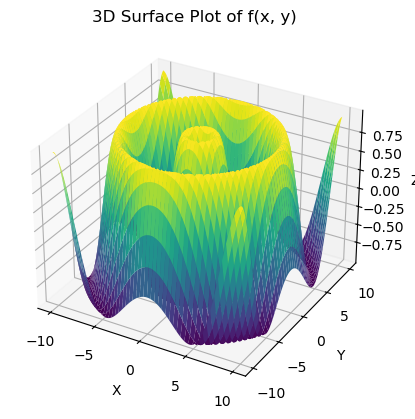
Questions
- If we can visualize a function of two variables as a surface, how do we visualize a function of three or more variables?
- Can we do math with functions of three or more variables?
For three variables \(\omega = f(x,y,z)\) we could use something called level surfaces, which are “slices” of the function where the \(\omega\) value is held constant. Kind of like a \(3D\) topographic map.
For more than three variables it is impossible to visualize using a graph, we just run out of axes in 3D space!
BUT we can absolutely do math no mater how many variables we have! This is the power of abstract thinking.
Functions of Two Variables
We will develop our ideas for functions of two variables, since they are easy to visualize, but remember these ideas will work no mater how many variables we have.
When we looked at the function
\[ z = x^2+y^2 \]
we could see that it has slope and curvature and even a minimum!
Partial Derivatives
Now that we are in two variables we might ask how the function changes if we were to walk in just one direction. Let’s look at our graph again.
def my_function(x, y):
    return x**2 + y**2  # I only made changes here

x = np.arange(-10, 10, .1)
y = np.arange(-10, 10, .1)
x, y = np.meshgrid(x, y)

z = my_function(x, y)

fig = plt.figure()
ax = fig.add_subplot(111, projection='3d')
ax.plot_surface(x, y, z, cmap='viridis')

ax.set_xlabel('X')
ax.set_ylabel('Y')
ax.set_zlabel('Z')
ax.set_title('3D Surface Plot of f(x, y)')
plt.show()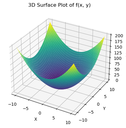
- If I started walking on the \(y=-10\) side (closest to us) and walked in a straight line along \(x=0\) what would my walk be like right at that moment?
I would be walking downhill!
- Could I say that the slope of a tangent line at that point in only the \(y\) direction would be negative?
Sure, works for me!
- What does this sound like?
Um… a derivative?
Partial Derivative in the \(y\) direction (and \(x\) direction)
We can define this idea EXACTLY like we did with the ordinary derivative. We just keep \(y\) as a constant and think about tangent lines going just in the \(y\) direction.
\[ \frac{\partial z}{\partial y} = \lim_{dy\to 0} \frac{f(x,y+dy) - f(x,y)}{dy} \]
But couldn’t we do the same thing in the \(x\) direction?
\[ \frac{\partial z}{\partial x} = \lim_{dx\to 0} \frac{f(x+dx,y) - f(x,y)}{dx} \]
# from IPython.display import Video

# # Animation code created by Google Gemini AI
# # Altered by Joanna
# # Let me know if you want to see this code!

# Video("tangent_animation_y.mp4")
Sympy can do these too!
# Enter the function
x,y = sp.symbols('x,y')
z = x**2+y**2
z
\(\displaystyle x^{2} + y^{2}\)
# Derivative with respect to y
sp.diff(z,y)
\(\displaystyle 2 y\)
# Derivative with respect to x
sp.diff(z,x)
\(\displaystyle 2 x\)
# Second derivative with respect to y
sp.diff(z,y,y)
\(\displaystyle 2\)
# Second derivative with respect to x
sp.diff(z,x,x)
\(\displaystyle 2\)
# Second derivative mixed x then y
sp.diff(z,x,y)
\(\displaystyle 0\)
# Second derivative mixed y then x
sp.diff(z,y,x)
\(\displaystyle 0\)
Interpreting the Partial Derivative
Just like with the ordinary derivative we are talking about slope. So we can see where the slope is negative or positive. But we can also look for maximums and minimums!
Question
- What was our process for finding critical points in functions of one variable?
- What might our process be now?
.
.
.
.
.
Critical Points
In this case we still want to look for where the slope is equal to zero, but now we have two slopes to consider:
\[\frac{\partial z}{\partial y} = 0 \]
and
\[\frac{\partial z}{\partial x} = 0 \]
in our example above
\[\frac{\partial z}{\partial y} = 2y = 0 \rightarrow y=0\]
\[\frac{\partial z}{\partial x} = 2x = 0 \rightarrow x=0 \]
so we have one critical point \((0,0,z(0,0)) = (0,0,0)\). Is this a max or a min?
We can look at the second derivatives!
Here is the notation for these second derivatives - which still talk about curvature:
\[ \frac{\partial^2 z}{\partial y^2} \]
\[ \frac{\partial^2 z}{\partial x^2} \]
\[ \frac{\partial^2 z}{\partial y \partial x} = \frac{\partial^2 z}{\partial x \partial y} \]
We have to consider all three of the partial derivatives to be sure we have a max or min. Here is the formula:
The determinant of the Hessian matrix (D) is calculated as:
\[ D = \frac{\partial^2 z}{\partial y^2}\frac{\partial^2 z}{\partial x^2} - \left(\frac{\partial^2 z}{\partial y \partial x}\right)^2 \]
- \(D > 0\) and \(\frac{\partial^2 z}{\partial x^2} > 0\): Local minimum
- \(D > 0\) and \(\frac{\partial^2 z}{\partial x^2} < 0\): Local maximum
- \(D < 0\): Saddle point
- \(D = 0\): Test is inconclusive
In our example:
\[D = (2)(2) - 0 > 0 \]
So we have a local minimum. This makes sense because we see that BOTH the second derivatives in \(x\) and \(y\) indicate that the function is concave up (valley) and the mixed partial derivative is not going to overcome this. FYI a non-zero mixed partial derivative indicates a kind of “twisting - curvature” in the surface.
Derivatives - Critical Points - Another Example
Consider the function
\[ z = 10x^2 - y^3 \]
- Plot the function
- Take the derivatives
- Interpret the derivatives and critical points.
def my_function(x, y):
    return 10*x**2 - y**3 # I made a change here!

x = np.arange(-10, 10, .1)
y = np.arange(-10, 10, .1)
x, y = np.meshgrid(x, y)

z = my_function(x, y)

fig = plt.figure()
ax = fig.add_subplot(111, projection='3d')
ax.plot_surface(x, y, z, cmap='viridis')

ax.set_xlabel('X')
ax.set_ylabel('Y')
ax.set_zlabel('Z')
ax.set_title('3D Surface Plot of f(x, y)')
plt.show()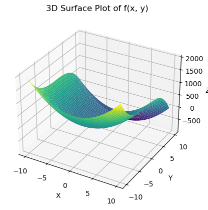
# Enter the function
x,y = sp.symbols('x,y')
z = 10*x**2-y**3
z
\(\displaystyle 10 x^{2} - y^{3}\)
# dz/dx
sp.diff(z,x)
\(\displaystyle 20 x\)
# dz/dy
sp.diff(z,y)
\(\displaystyle - 3 y^{2}\)
# d2z/dx2
sp.diff(z,x,x)
\(\displaystyle 20\)
# d2z/dxdy
sp.diff(z,x,y)
\(\displaystyle 0\)
# d2x/xy2
sp.diff(z,y,y)
\(\displaystyle - 6 y\)
Interpret the results:
To have a critical point I would need BOTH \(2x=0\) and \(-3y^2=0\). This happens when \(x=y=0\) or at the point \((0,0,0)\).
I have to decide if this is a maximum or minimum - look at the second derivatives and plug in the critical points! The second derivative in x is positive, but the other two are zero. This means that \(D=0\) so we have a Saddle Point
Saddle Point Saddle points are points where the function is s-shaped in one direction and u-shaped in the other but the slope right in the middle is zero. Look back at the graph. In the x-direction we do have a minimum, but in the y-direction it is the flat part of the s-shape.
To have a verified maximum or minimum we would need BOTH directions to be conclusive.
Application - Remember Least Squares?
Remember when we were doing linear regression and we said we needed to minimize the mean squared error… here is a reminder:
The goal is to minimize the sum of square distances between the line \(\hat{y}=\beta_0+\beta_1x\) and the data point values \(y\). Lets look at this is parts:
- What is the distance between \(y\) and \(\hat{y}\) for each point in the data?
\[y_i - \hat{y}_i = y_i - (\beta_0+\beta_1x_i)\]
This is also called the residual or error for point \(i\) in our data.
- What is the square distance?
\[(y_i - (\beta_0+\beta_1x_i))^2\]
We just square the residual or error for point \(i\) in our data.
- How do we add these up?
Using the summation notation:
\[\sum_i (y_i - (\beta_0+\beta_1x_i))^2\]
Now we are adding up the square error for all of the points in the data.
- How can we minimize this?
We need to choose \(\beta_0\) and \(\beta_1\) that are a minimum for this function. Lets look at the function for our example data.
Imagine we just have two data points:
We will plot our data, look at our sum of square errors, and then try to find a minimum!
np.random.seed(0)
xdata = np.arange(0,1,.5)
noise = np.random.rand(len(xdata))
ydata = xdata+noise

plt.plot(xdata,ydata,'k.')
plt.xlabel('x')
plt.ylabel('y')
plt.show()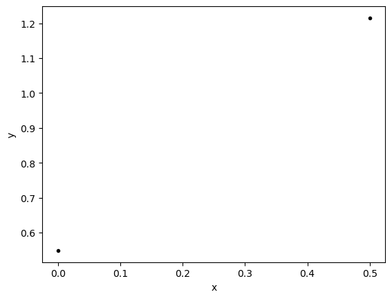
# Create the symbols
b0, b1 = sp.symbols('b0,b1')
# Define the function to plot
f = 0
for x,y in zip(xdata,ydata):
    f = f + (y-(b0 + b1*x))**2
# Look at the function
f
\(\displaystyle \left(0.548813503927325 - b_{0}\right)^{2} + 1.4766851961446 \left(- 0.822917010033751 b_{0} - 0.411458505016876 b_{1} + 1\right)^{2}\)
This is a function of two variables and we are looking for a minimum, \(f = f(\beta_0,\beta_1)\).
We will plot this function and then find the critical points!
def least_square(beta0, beta1):
    return (0.548813503927325 - beta0)**2 + 1.4766851961446*(-0.822917010033751*beta0 - 0.411458505016876*beta1 + 1)**2

x = np.arange(-5, 5, .1)
y = np.arange(-5, 5, .1)
x, y = np.meshgrid(x, y)

z = least_square(x, y)

fig = plt.figure()
ax = fig.add_subplot(111, projection='3d')
ax.plot_surface(x, y, z, cmap='viridis')

ax.set_xlabel('beta_0')
ax.set_ylabel('beta_1')
ax.set_zlabel('Z')
ax.set_title('3D Surface Plot of f(x, y)')
plt.show()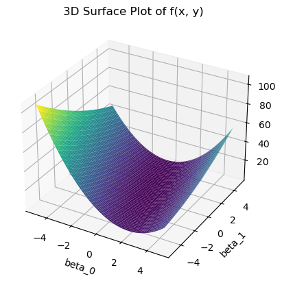
Does the least squares function have a minimum?
We can check - but YES - this is a special kind of function a quadratic and it will have a max or min. Let’s do the math!
sp.diff(f,b0)\(\displaystyle 4.0 b_{0} + 1.0 b_{1} - 3.52800574059949\)
sp.diff(f,b1)\(\displaystyle 1.0 b_{0} + 0.5 b_{1} - 1.21518936637242\)
sp.diff(f,b0,b0)\(\displaystyle 4.0\)
sp.diff(f,b1,b1)\(\displaystyle 0.5\)
sp.diff(f,b0,b1)\(\displaystyle 1.0\)
Are there critical points? Well we need two equations to be equal to zero
\[4.0*b0 + 1.0*b1 - 3.52800574059949=0\] \[1.0*b0 + 0.5*b1 - 1.21518936637242=0\]
Lets use sympy to solve this.
eqn1 = 4*b0 + 1*b1 - 3.52800574059949
eqn2 = 1*b0 + 0.5*b1 - 1.21518936637242

sp.solve([eqn1,eqn2],[b0,b1])
{b0: 0.548813503927325, b1: 1.33275172489019}We found a critical point! \(\beta_0 = 0.548813503927325\) and \(\beta_1 = 1.33275172489019\). Is this a max, min, or saddle?
\[D = (4)(0.5) - 1 = 1 > 0 \]
\[\frac{\partial^2 z}{\partial x^2} > 0 \]
So this is a minimum. These values of \(\beta\) minimize the square error function and they should be the line of best fit for our data:
\[ y = \beta_0 + \beta_1 x = 0.548813503927325 + 1.33275172489019 x \]
Lets look at the graph
yfit = 0.548813503927325 + 1.33275172489019*xdata

plt.plot(xdata,ydata,'k.')
plt.plot(xdata,yfit,'-r')
plt.xlabel('x')
plt.ylabel('y')
plt.show()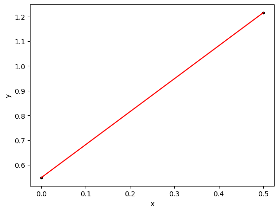
IT WORKED!!!
Now we can do this same thing for even more points!
np.random.seed(0)
xdata = np.arange(0,1,.01)
noise = np.random.rand(len(xdata))
ydata = xdata+noise

plt.plot(xdata,ydata,'k.')
plt.xlabel('x')
plt.ylabel('y')
plt.show()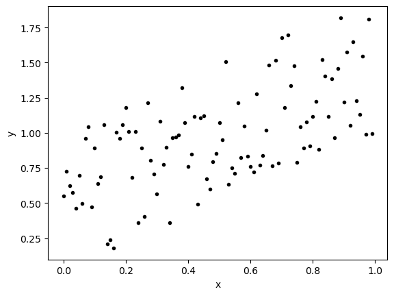
# Create the symbols
b0, b1 = sp.symbols('b0,b1')
# Define the function to plot
f = 0
for x,y in zip(xdata,ydata):
    f = f + (y-(b0 + b1*x))**2
# Look at the function
f
\(\displaystyle \left(0.548813503927325 - b_{0}\right)^{2} + \left(- b_{0} - 0.99 b_{1} + 0.994695476192547\right)^{2} + \left(- b_{0} - 0.97 b_{1} + 0.990107546187494\right)^{2} + \left(- b_{0} - 0.87 b_{1} + 0.963940510758442\right)^{2} + \left(- b_{0} - 0.82 b_{1} + 0.884147496348784\right)^{2} + \left(- b_{0} - 0.79 b_{1} + 0.908727718954244\right)^{2} + \left(- b_{0} - 0.77 b_{1} + 0.890196561213169\right)^{2} + \left(- b_{0} - 0.75 b_{1} + 0.789187792254321\right)^{2} + \left(- b_{0} - 0.69 b_{1} + 0.786098407893963\right)^{2} + \left(- b_{0} - 0.67 b_{1} + 0.767101275793061\right)^{2} + \left(- b_{0} - 0.64 b_{1} + 0.836582361680054\right)^{2} + \left(- b_{0} - 0.63 b_{1} + 0.768182951348614\right)^{2} + \left(- b_{0} - 0.61 b_{1} + 0.720375141164305\right)^{2} + \left(- b_{0} - 0.6 b_{1} + 0.75896958364552\right)^{2} + \left(- b_{0} - 0.59 b_{1} + 0.834425592001603\right)^{2} + \left(- b_{0} - 0.57 b_{1} + 0.823291602539782\right)^{2} + \left(- b_{0} - 0.55 b_{1} + 0.711309517884996\right)^{2} + \left(- b_{0} - 0.54 b_{1} + 0.748876756094835\right)^{2} + \left(- b_{0} - 0.53 b_{1} + 0.632044810748028\right)^{2} + \left(- b_{0} - 0.51 b_{1} + 0.94860151346232\right)^{2} + \left(- b_{0} - 0.49 b_{1} + 0.853710770942623\right)^{2} + \left(- b_{0} - 0.48 b_{1} + 0.795428350924184\right)^{2} + \left(- b_{0} - 0.47 b_{1} + 0.598926297654853\right)^{2} + \left(- b_{0} - 0.46 b_{1} + 0.670382561073841\right)^{2} + \left(- b_{0} - 0.43 b_{1} + 0.49022547162927\right)^{2} + \left(- b_{0} - 0.41 b_{1} + 0.847031953799341\right)^{2} + \left(- b_{0} - 0.4 b_{1} + 0.759507900573786\right)^{2} + \left(- b_{0} - 0.37 b_{1} + 0.986933996874757\right)^{2} + \left(- b_{0} - 0.36 b_{1} + 0.972095722722421\right)^{2} + \left(- b_{0} - 0.35 b_{1} + 0.967635497075877\right)^{2} + \left(- b_{0} - 0.34 b_{1} + 0.358789800436355\right)^{2} + \left(- b_{0} - 0.33 b_{1} + 0.898433948868649\right)^{2} + \left(- b_{0} - 0.32 b_{1} + 0.776150332216549\right)^{2} + \left(- b_{0} - 0.3 b_{1} + 0.564555612104627\right)^{2} + \left(- b_{0} - 0.29 b_{1} + 0.704661939990524\right)^{2} + \left(- b_{0} - 0.28 b_{1} + 0.801848321750072\right)^{2} + \left(- b_{0} - 0.26 b_{1} + 0.403353287409046\right)^{2} + \left(- b_{0} - 0.25 b_{1} + 0.889921021327524\right)^{2} + \left(- b_{0} - 0.24 b_{1} + 0.358274425868933\right)^{2} + \left(- b_{0} - 0.22 b_{1} + 0.681479362252932\right)^{2} + \left(- b_{0} - 0.18 b_{1} + 0.958156750949851\right)^{2} + \left(- b_{0} - 0.16 b_{1} + 0.180218397440326\right)^{2} + \left(- b_{0} - 0.15 b_{1} + 0.237129299701541\right)^{2} + \left(- b_{0} - 0.14 b_{1} + 0.211036058197887\right)^{2} + \left(- b_{0} - 0.12 b_{1} + 0.688044561093932\right)^{2} + \left(- b_{0} - 0.11 b_{1} + 0.638894919752904\right)^{2} + \left(- b_{0} - 0.1 b_{1} + 0.891725038082665\right)^{2} + \left(- b_{0} - 0.09 b_{1} + 0.473441518825778\right)^{2} + \left(- b_{0} - 0.07 b_{1} + 0.96177300078208\right)^{2} + \left(- b_{0} - 0.06 b_{1} + 0.497587211262693\right)^{2} + \left(- b_{0} - 0.05 b_{1} + 0.695894113066656\right)^{2} + \left(- b_{0} - 0.04 b_{1} + 0.463654799338905\right)^{2} + \left(- b_{0} - 0.03 b_{1} + 0.574883182996897\right)^{2} + \left(- b_{0} - 0.02 b_{1} + 0.622763376071644\right)^{2} + \left(- b_{0} - 0.01 b_{1} + 0.725189366372419\right)^{2} + 1.00524655468657 \left(- 0.997387000108195 b_{0} - 0.169555790018393 b_{1} + 1\right)^{2} + 1.01840100773196 \left(- 0.990924553839731 b_{0} - 0.208094156306343 b_{1} + 1\right)^{2} + 1.02116921612618 \left(- 0.989580532127584 b_{0} - 0.227603522389344 b_{1} + 1\right)^{2} + 1.03780097333821 \left(- 0.981619016393975 b_{0} - 0.638052360656084 b_{1} + 1\right)^{2} + 1.08744636119784 \left(- 0.958950252431525 b_{0} - 0.728802191847959 b_{1} + 1\right)^{2} + 1.08923195765663 \left(- 0.958163918313931 b_{0} - 0.0766531134651145 b_{1} + 1\right)^{2} + 1.09476623339516 \left(- 0.955738988780663 b_{0} - 0.554328613492785 b_{1} + 1\right)^{2} + 1.10627874335845 \left(- 0.950753025599441 b_{0} - 0.874692783551485 b_{1} + 1\right)^{2} + 1.11428426277477 \left(- 0.947331550446595 b_{0} - 0.123153101558057 b_{1} + 1\right)^{2} + 1.12362575443084 \left(- 0.943385414642582 b_{0} - 0.179243228782091 b_{1} + 1\right)^{2} + 1.14532112741286 \left(- 0.934407603948879 b_{0} - 0.46720380197444 b_{1} + 1\right)^{2} + 1.14879875357028 \left(- 0.932992219718588 b_{0} - 0.363866965690249 b_{1} + 1\right)^{2} + 1.158077724723 \left(- 0.929246953419767 b_{0} - 0.724812623667419 b_{1} + 1\right)^{2} + 1.17556269330413 \left(- 0.922310392810085 b_{0} - 0.285916221771126 b_{1} + 1\right)^{2} + 1.22493256241839 \left(- 0.903532773478216 b_{0} - 0.397554420330415 b_{1} + 1\right)^{2} + 1.24409371649816 \left(- 0.89654780515974 b_{0} - 0.762065634385779 b_{1} + 1\right)^{2} + 1.24909949010981 \left(- 0.894749541390825 b_{0} - 0.375794807384147 b_{1} + 1\right)^{2} + 1.24988638940786 \left(- 0.894467840331971 b_{0} - 0.715574272265577 b_{1} + 1\right)^{2} + 1.25582923482233 \left(- 0.8923489265455 b_{0} - 0.401557016945475 b_{1} + 1\right)^{2} + 1.28412266292754 \left(- 0.88246348633367 b_{0} - 0.838340312016986 b_{1} + 1\right)^{2} + 1.38914119664751 \left(- 0.848451075439407 b_{0} - 0.169690215087881 b_{1} + 1\right)^{2} + 1.38921865514557 \left(- 0.848427421617222 b_{0} - 0.602383469348228 b_{1} + 1\right)^{2} + 1.47163180931346 \left(- 0.824328692671661 b_{0} - 0.46162406789613 b_{1} + 1\right)^{2} + 1.47542057804641 \left(- 0.823269605374432 b_{0} - 0.222282793451097 b_{1} + 1\right)^{2} + 1.48491029187832 \left(- 0.820634727307272 b_{0} - 0.738571254576545 b_{1} + 1\right)^{2} + 1.49881987973803 \left(- 0.816817958625325 b_{0} - 0.661622546486513 b_{1} + 1\right)^{2} + 1.5114393413757 \left(- 0.81340088172391 b_{0} - 0.764596828820475 b_{1} + 1\right)^{2} + 1.62901722094459 \left(- 0.783496683187417 b_{0} - 0.485767943576199 b_{1} + 1\right)^{2} + 1.75230897537116 \left(- 0.755430747157041 b_{0} - 0.287063683919676 b_{1} + 1\right)^{2} + 1.78181256158342 \left(- 0.74915035875537 b_{0} - 0.54687976189142 b_{1} + 1\right)^{2} + 1.91337517741941 \left(- 0.722936133901506 b_{0} - 0.621725075155296 b_{1} + 1\right)^{2} + 1.97852765097605 \left(- 0.710933432501015 b_{0} - 0.597184083300853 b_{1} + 1\right)^{2} + 2.11978019792232 \left(- 0.686838426447803 b_{0} - 0.604417815274067 b_{1} + 1\right)^{2} + 2.18822073733428 \left(- 0.676012046755559 b_{0} - 0.500248914599113 b_{1} + 1\right)^{2} + 2.19334094685542 \left(- 0.675222532990699 b_{0} - 0.445646871773862 b_{1} + 1\right)^{2} + 2.27519163534152 \left(- 0.662965622160794 b_{0} - 0.344742123523613 b_{1} + 1\right)^{2} + 2.30415674220155 \left(- 0.658785437508237 b_{0} - 0.447974097505601 b_{1} + 1\right)^{2} + 2.31792135425904 \left(- 0.656826477987516 b_{0} - 0.545165976729639 b_{1} + 1\right)^{2} + 2.3917022575349 \left(- 0.64661599492073 b_{0} - 0.620751355123901 b_{1} + 1\right)^{2} + 2.48822350681717 \left(- 0.633950437186184 b_{0} - 0.576894897839427 b_{1} + 1\right)^{2} + 2.71039326302085 \left(- 0.60741266833126 b_{0} - 0.564893781548071 b_{1} + 1\right)^{2} + 2.810516337833 \left(- 0.596495185758643 b_{0} - 0.41754663003105 b_{1} + 1\right)^{2} + 2.87899819039686 \left(- 0.589358164187122 b_{0} - 0.424337878214728 b_{1} + 1\right)^{2} + 3.27226402930491 \left(- 0.552809923960083 b_{0} - 0.541753725480881 b_{1} + 1\right)^{2} + 3.30983865451527 \left(- 0.549663106718008 b_{0} - 0.489200164979027 b_{1} + 1\right)^{2}\)
This looks scary, but look closer! This is just a function of two variables! We could do the same thing:
- Take partial derivatives.
- Find critical points.
- Check if there is a max or min.
And if we look at a plot it does have the same quadratic shape!
sp.plotting.plot3d(f)
plt.show()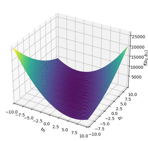
This is where we got those formulas that are used for general least squares!
\[\beta_1 = \frac{n\sum_i x_iy_i-\sum_i x_i\sum_iy_i}{n\sum_ix_i^2-(\sum_ix_i)^2)}\]
\[\beta_0= \bar{y}-\beta_1\bar{x}\]
where \(\bar{x}\) and \(\bar{y}\) are the averages of the \(x_i\) and \(y_i\) data points respectively.
You Try
Find all the critical points and classify them as maximum, minimum, or saddle using the partial derivative.
Number 1 \[ z = 5 e^{-(x^2 + 2*y^2)} \]
Number 2 \[ z = -x^4 + 4x^2 - y^2 (x - 1.5)\] for this one I changed my x and y range in the graph a few times \([-2,2]\),\([-5,5]\),\([-10,10]\), this gave a much better view of the function!
Copy and paste the 3d plotting code and use it to plot the function.
- You might need to change the range of x and y to get the best view of the function
Enter the function using sympy
Take all the derivatives
Find any critical points
- Use sp.solve() to find where the first derivative equations are zero
- Ignore any answers with imaginary numbers
- It is okay to get more than one critical point!
Classify them as global/local/max/min using \(D\)
- If you have more than one critical point, you will have to calculate \(D\) separately for each one
- Remember to plug the critical point into your derivatives
dxx = diff(f,x,x) # Take the derivaitve dxx.subs({x:0,y:0}) # Plug in x=0 AND y=0- Then plug those values into \(D\)
Find the value of your function at the critical point - sub in the critical point
z.subs({x:0,y:0})Interpret your results
You can see my solutions below but please try to figure these out without looking! At the beginning of the next class you will do an example of this on your own as part of practicing for Exam2
Solution to number 1
# Plot the function
def my_function(x, y):
    return 5*np.exp(-(x**2+2*y**2)) # I made a change here!

x = np.arange(-10, 10, .1)
y = np.arange(-10, 10, .1)
x, y = np.meshgrid(x, y)

z = my_function(x, y)

fig = plt.figure()
ax = fig.add_subplot(111, projection='3d')
ax.plot_surface(x, y, z, cmap='viridis')

ax.set_xlabel('X')
ax.set_ylabel('Y')
ax.set_zlabel('Z')
ax.set_title('3D Surface Plot of f(x, y)')
plt.show()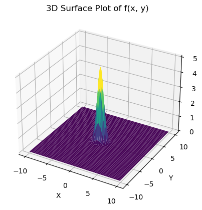
# Enter the function into Sympy
x,y = sp.symbols('x,y')
z = 5*sp.exp(-(x**2+2*y**2))
z
\(\displaystyle 5 e^{- x^{2} - 2 y^{2}}\)
# Calculate all the derivatives and print them out
print(sp.diff(z,x))
print(sp.diff(z,y))
-10*x*exp(-x**2 - 2*y**2)
-20*y*exp(-x**2 - 2*y**2)# Copy and paste the first two equations
# This are my first derivatives
# Solve for what values of x and y make these both zero
eqn1 = -10*x*sp.exp(-x**2 - 2*y**2)
eqn2 = -20*y*sp.exp(-x**2 - 2*y**2)
sp.solve([eqn1,eqn2],[x,y]){x: 0, y: 0}# Copy and paste the third equation - second derivative in x
# Sub in the critical point
dxx = sp.diff(z,x,x)
dxx.subs({x:0,y:0})\(\displaystyle -10\)
# Copy and paste the fourth equation - second derivative in y
# Sub in the critical point
dyy = sp.diff(z,y,y)
dyy.subs({x:0,y:0})
\(\displaystyle -20\)
# Copy and past the fourth equation - mixed partial derivative
# Sub in the critical point
dxy = sp.diff(z,x,y)
dxy.subs({x:0,y:0})
\(\displaystyle 0\)
# Calculate D
D = (-10)*(-20)-0
D200# Sub the critical point into the origial function
# This gives us the value of the maximum
z.subs({x:0,y:0})\(\displaystyle 5\)
Interpret Results
I have a max value at \(x=0\), \(y=0\). At that point \(z=5\)
This is a global max, because we have a decaying exponential. As \(x\) and \(y\) go to infinity our function goes to zero.
Solution to number 2
# Plot the function
def my_function(x, y):
    return -x**4 + 4*x**2 - y**2 * (x - 1.5) # I made a change here!

x = np.arange(-2, 2, .1)
y = np.arange(-2, 2, .1)
x, y = np.meshgrid(x, y)

z = my_function(x, y)

fig = plt.figure()
ax = fig.add_subplot(111, projection='3d')
ax.plot_surface(x, y, z, cmap='viridis')

ax.set_xlabel('X')
ax.set_ylabel('Y')
ax.set_zlabel('Z')
ax.set_title('3D Surface Plot of f(x, y)')
plt.show()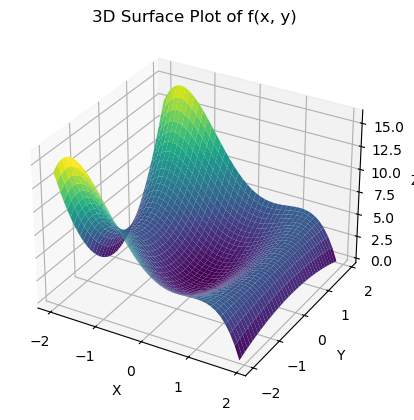
x,y = sp.symbols('x,y')
z = -x**4 + 4*x**2 - y**2 * (x - 1.5)
z
\(\displaystyle - x^{4} + 4 x^{2} - y^{2} \left(x - 1.5\right)\)
print(sp.diff(z,x))
print(sp.diff(z,y))
-4*x**3 + 8*x - y**2
-2*y*(x - 1.5)# Copy and paste from above
eqn1 = 4*x**3 + 8*x - y**2
eqn2 = -2*y*(x - 1.5)
sp.solve([eqn1,eqn2],[x,y])[(0.0, 0.0),
(1.50000000000000, -5.04975246918104),
(1.50000000000000, 5.04975246918104),
(-1.4142135623731*I, 0.0),
(1.4142135623731*I, 0.0)]I have more than one critical point!
\((0,0)\), \((1.50000000000000, -5.04975246918104)\), and \((1.50000000000000, 5.04975246918104)\)
I will have to test these individually to see if they are max, min, or saddle!
Start with (0,0)
critical_point = {x:0,y:0}
print(f'diff_xx: {sp.diff(z,x,x).subs(critical_point)}')
print(f'diff_yy: {sp.diff(z,y,y).subs(critical_point)}')
print(f'diff_xy: {sp.diff(z,x,y).subs(critical_point)}')
print(f'z: {z.subs(critical_point)}')
D = sp.diff(z,x,x).subs(critical_point)*sp.diff(z,y,y).subs(critical_point) - sp.diff(z,x,y).subs(critical_point)**2
print(f'D: {D}')
diff_xx: 8
diff_yy: 3.00000000000000
diff_xy: 0
z: 0
D: 24.0000000000000Then do (1.50000000000000, -5.04975246918104)
critical_point = {x:1.50000000000000,y:-5.04975246918104}
print(f'diff_xx: {sp.diff(z,x,x).subs(critical_point)}')
print(f'diff_yy: {sp.diff(z,y,y).subs(critical_point)}')
print(f'diff_xy: {sp.diff(z,x,y).subs(critical_point)}')
print(f'z: {z.subs(critical_point)}')
D = sp.diff(z,x,x).subs(critical_point)*sp.diff(z,y,y).subs(critical_point) - sp.diff(z,x,y).subs(critical_point)**2
print(f'D: {D}')
diff_xx: -19.0000000000000
diff_yy: 0
diff_xy: 10.0995049383621
z: 3.93750000000000
D: -102.000000000000Then do (1.50000000000000, 5.04975246918104)
critical_point = {x:1.50000000000000,y:5.04975246918104}
print(f'diff_xx: {sp.diff(z,x,x).subs(critical_point)}')
print(f'diff_yy: {sp.diff(z,y,y).subs(critical_point)}')
print(f'diff_xy: {sp.diff(z,x,y).subs(critical_point)}')
print(f'z: {z.subs(critical_point)}')
D = sp.diff(z,x,x).subs(critical_point)*sp.diff(z,y,y).subs(critical_point) - sp.diff(z,x,y).subs(critical_point)**2
print(f'D: {D}')
diff_xx: -19.0000000000000
diff_yy: 0
diff_xy: -10.0995049383621
z: 3.93750000000000
D: -102.000000000000Interpret the results
I can see that \((0,0)\) is a minimum since D is positive and the second derivative in x in positive. The other two points are both maximums since D is positive and the second derivative in x is negative. The two maxes are tied for global max. The minimum is just a local minimum since the function goes to minus infinity in other areas.