# We will just go ahead and import all the useful packages first.
import numpy as np
import sympy as sp
import pandas as pd
import matplotlib.pyplot as plt
from mpl_toolkits.mplot3d import Axes3D

# Special Functions
from sklearn.metrics import r2_score, mean_squared_error

## NEW
from scipy.stats import binom, beta

# Functions to deal with dates
import datetimeMath for Data Science
Probability Distributions
Important Information
- Email: joanna_bieri@redlands.edu
- Office Hours take place in Duke 209 unless otherwise noted – Office Hours Schedule
Today’s Goals:
- Introduction to Probability Distributions.
- Binomial Distribution
- Beta Distribution
(Review) Probability
We express the idea of probability as
\[P(X)\] where \(X\) is the event of interest.
(Review) Conditional Probabilities
\[P(A\; given\; B) = P(A|B)\]
Pop Quiz
- What does the conditional probability calculate - give an example (eg we did cancer and coffee)
- What is the difference between independent and dependent events in probability?
Joint Probability
\[P(A\; and\; B) = P(B) \times P(A|B) \]
Pop Quiz
- What is this formula used to calculate - say in your own words.
- How does this formula change if \(A\) and \(B\) are independent events?
Union Probability.
\[P(A\; or\; B) = P(A)+P(B) - P(B) \times P(A|B))\]
Pop Quiz
- What is this formula used to calculate - say in your own words.
- Why do we subtract off the Joint Probability?
- How does this formula change if \(A\) and \(B\) are independent events?
(Review) Bayes’ Theorem
\[ P(A|B) = \frac{P(B|A)P(A)}{P(B)} = P(B|A)\frac{P(A)}{P(B)}\]
Pop Quiz
- What does Bayes’ Theorem do for our conditional probabilities?
- If event \(A\) is your team winning the Champions League and event \(B\) is your team scoring an average of 2.5 points per game. What does \(P(B|A)\) mean in words and what does Bayes theorem let you do?
Probability Distributions
A probability distribution is a mathematical function that gives the probabilities of events occurring for a range of possible event outcomes. Instead of being able to represent mathematically a single event (the probability of rolling a 6 on a fair die) we can think about representing all possible events (the probability of rolling a 1,2,3,4,5,6 on a fair die) using a single function or graph.
Probability distributions can be defined in different ways and for discrete or for continuous variables.
discrete only specific outcomes can occur: yes/no, heads/tails, 1/2/3/4/5/6, integer values.
continuous a continuous range of outcomes can occur: height, weight, temperature, real values.
Distributions with special properties or for important applications are given special names. We will discuss a few of these distributions that are most important to data science and machine learning.
Binomial Distribution
The binomial distribution helps us model the probability that we would have \(k\) successes given \(n\) independent trials.
Example Here is an example of the use of this idea: What is the probability that we would get 5 heads if we flipped a fair coin 8 times in a row.
Assume we have \(n\) independent Bernoulli trials, where each trial has a probability \(p\) of success. The probability of \(k\) successes is given by
\[P(X = k) = \binom{n}{k} p^k (1-p)^{n-k}\]
where:
- \(n\) is the number of trials
- \(k\) is the number of successes (\(0 \le k \le n\))
- \(p\) is the probability of success in a single trial
- \[\binom{n}{k} = \frac{n!}{k!(n-k)!}\] is the binomial coefficient, representing the number of ways to choose \(k\) successes from \(n\) trials.
Here \(P(X = k)\) is a probability mass function. If we find it’s values across all possible values of \(k\) then we would produce the Binomial Distribution.
Apply this to the Example
- An independent Bernoulli trial in this case is a single flip of the coin. The characteristics of a Bernouli trial are:
- The events are independent - one flip of the coin does not effect the next
- There are two possible outcomes - success or failure - heads or tails
- The probability of success remains constant - probability does not change as we are doing the trials.
- The number of trials we would do is \(n=8\) - we are flipping the coin 8 times in a row
- The number of successes we are looking for is \(k=5\) - probability of getting 5 heads
- The probability of success is \(p=0.5\) - 50% probability of flipping heads
Plugging into the formula would look like this:
Find the binomial coefficient will tell us the number of ways we can get 5 heads given that we flip the coin 8 times. We also say “8 choose 5”:
\[\binom{8}{5} = \frac{8!}{5!(8-5)!} = \frac{8*7*6*5*4*3*2*1}{(5*4*3*2*1)(3*2*1)} = \frac{8*7*6}{3*2*1} = \frac{336}{6} = 56\]
Plug into the function:
\[P(X = 5) = \binom{8}{5} (0.5)^5 (1-0.5)^{8-5} = 56(0.5)^5(0.5)^3 = 0.21875\]
Some things to note:
- This formula takes advantage of the idea that if \(p\) is the probability of success then \(1-p\) is the probability of failure.
- We calculated the formula for just one example outcome.
- We can ask Python to do this for us!
n = 8
p = 0.5
k = 5

# Above we imported a new package for the binomial distribution
from scipy.stats import binom

# Then we will use the PMF function - Probability Mass Function
# We need to send things in in the correct order!
binom.pmf(k,n,p)0.2187499999999999So we have a 21.87% chance of flipping heads five times out of a total of 8 flips.
How is this related to the Binomial Distribution. The probability distribution is a plot/representation of all the possible outcomes or events, so we would have to calculate all of these cases \(k = 0,1,2,3,4,5,6,7,8\). This would result in a discrete probability distribution.
n = 8 # Number of Trials
p = 0.5 # Probability of Success

flip_binom = []
k_vals = []
for k in range(n+1):
    k_vals.append(k)
    P = binom.pmf(k,n,p)
    flip_binom.append(P)
    print(f'k={k}:   P(X={k})={P}')

plt.bar(k_vals,flip_binom)
plt.title('A Binomial Distribuion')
plt.xlabel(f'k outcomes in n={n} trials')
plt.ylabel('Probability')
plt.show()
k=0: P(X=0)=0.003906250000000007
k=1: P(X=1)=0.031249999999999983
k=2: P(X=2)=0.10937500000000004
k=3: P(X=3)=0.21874999999999992
k=4: P(X=4)=0.27343749999999994
k=5: P(X=5)=0.2187499999999999
k=6: P(X=6)=0.10937500000000004
k=7: P(X=7)=0.031249999999999983
k=8: P(X=8)=0.00390625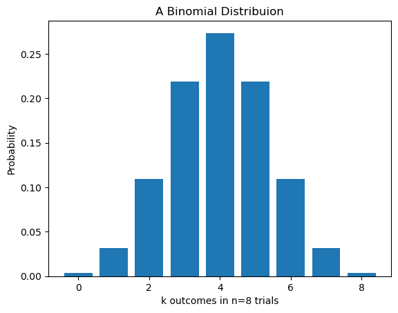
Interpret these Results
- The highest probability event is that we get 4 heads in 8 flips. It has a probability of 27.34%.
- Lowest probabilities are flipping either no heads or 8 heads in 8 flips. This makes sense.
- If I add up all of the probabilities I should get 1. There is 100% chance that I got one of these outcomes if I flipped a coin 8 times!
sum(flip_binom)0.9999999999999998What happened here?
Well we lost our perfect number to rounding! This in an unfortunate consequence of using a computer to do mathematical calculations for us. Be aware of rounding and chopping errors when using computers to do calculations You should make sure that your calculations are not sensitive to this amount of error.
Binomial Distribution - Another Example
Adapted from our book: Essential Math for Data Science
Imagine that you are working on a new turbine jet engine and testing the engine is very expensive! You want to run a limited number of tests and hope to get at least a 90% success rate in your testing to prove that your design is worth continued research. If you have less than 90% success rates in your experiments then it is back to the drawing board for a complete redesign.
Here are your results
data = {
    'Experiment': [1,2,3,4,5,6,7,8,9,10],
    'Outcome': ['Pass','Pass','Pass','Pass','Pass','Fail','Pass','Fail','Pass','Pass']
}

DF = pd.DataFrame(data)
DF| Experiment | Outcome | |
|---|---|---|
| 0 | 1 | Pass |
| 1 | 2 | Pass |
| 2 | 3 | Pass |
| 3 | 4 | Pass |
| 4 | 5 | Pass |
| 5 | 6 | Fail |
| 6 | 7 | Pass |
| 7 | 8 | Fail |
| 8 | 9 | Pass |
| 9 | 10 | Pass |
Just looking at this data - what does the likelihood say about your marginal probability of success?
\[P(Pass) = 0.80\]
Now there are a few ways of thinking about this data:
- We are only getting an 80% success rate, it is back to the drawing board for us!
- If we did just a few more experiments would would probably hit our goal of 90% success.
What do you think? Did we do enough experiments? How many more should we do?
The argument here is that if you flip a fair coin 10 times you will most likely get 5 heads, but this is not a guarantee! You might get more or fewer.
What we want to know here is if the underlying probability of success really is 90% then what is the probability that we got 8 successes in 10 tries?
You Try - Binomial Distribution
- Assuming we really do have an underlying 90% success rate, calculate the probability that we see 8 successes in just 10 tests of our engine. Use the Binomial PMF (probability mass function)
- Find and plot the the Binomial Distribution for this example. We have 10 trials and are assuming a probability of success of 90%.
# Your code here# Your code hereHERE IS JOANNA’S CODE - MAKE SURE YOU TRY ON YOUR OWN FIRST
Code
n = 10 # Number of Trials
p = 0.9 # Probability of Success
K = 8 # Focal number of successes

print("Joanna's Results")

engine_binom = []
k_vals = []
for k in range(n+1):
    k_vals.append(k)
    P = binom.pmf(k,n,p)
    engine_binom.append(P)
    if k==K:
        print(f'The probability of {k} successes in {n} experiments is P(X={k})={P}')

plt.bar(k_vals,engine_binom)
plt.title('A Binomial Distribuion - Engine Example')
for i, value in enumerate(engine_binom):
    plt.text(i, value, str(round(value,4)), ha='center', va='bottom',rotation=45) # Adjust vertical offset (+1) as needed

plt.xlabel(f'k outcomes in n={n} trials')
plt.ylabel('Probability')
plt.show()
Joanna's Results
The probability of 8 successes in 10 experiments is P(X=8)=0.1937102444999998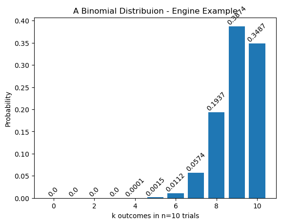
Interpret our Results
First we see that we have a 19.37% probability of seeing 8 successful trials in 10 tries if we have an underlying success rate of 90%. It is much less likely that we would have only 1 or 2 successes. In fact those numbers are so small the are essentially zero!
How could we calculate the probability that we had 8 or fewer successes? This is like asking what is the probability that I had 0 or 1 or 2 or….. or 8 successes. I hope this sounds like a union probability! We can add these up and we can’t get both 0 and 1 so they are independent.
start = 0
end = 8

# Here we are adding up the values in our list
# We start at zero and we go until 8+1 to get all the values in the list
sum(engine_binom[start:end+1])0.26390107089999976So in our engine experiments there is actually at 26.39% chance that we would see 8 or fewer successes in just 10 experiments even if we had a 90% success rate for our engines. Maybe it is worth it to run a few more experiments before scrapping our design!
One big underlying assumption throughout this modeling process is that the underlying success rate was actually 90%. As long as we are clear about this assumption these results are still good. But it is worth considering… what if our underlying probability of success were actually different?
Beta Distribution
Continuing to think about the engine example above, how could I flip my question around a bit to explore the fact that we might have a different underlying probability of success? Instead lets ask
What other underlying rates of success might yield 8 successes in 10 trials
In this case we want to fix the success rate - what we saw experimentally - and explore the probability of the underlying probabilities. Now there are a few ways we could do this:
- BRUTE FORCE - create a new binomial distribution for every possible underlying probability and compare them. Wow this is a lot of work!
- MATH TO THE RESCUE - learn about the Beta Distribution - which calculates the likelihood of different underlying probabilities.
I am lazy - I’ll do math all day to avoid doing “real: work :)
The beta distribution is a continuous probability distribution. The x-axis of the beta distribution goes from \([0, 1]\) and represents underlying rates of success between 0% and 100%. It has two parameters, \(\alpha\) (the number of successes) and \(\beta\) (the number of failures). Since beta is a continuous probability distribution we have to be a little careful in how we interpret results. Let’s first look at a graph and talk about the ideas and then define the function.
alpha_val = 8
beta_val = 2

# This is the new package that we imported above
from scipy.stats import beta

# Generate x values (range from 0 to 1)
x = np.linspace(0, 1, 100)

# Calculate the probability density function (PDF)
pdf = beta.pdf(x, alpha_val, beta_val)

plt.plot(x,pdf,'-k')
plt.title(f'beta Distribution with alpha={alpha_val} and beta={beta_val}')
plt.xlabel('Underlying Rate of Success')
plt.ylabel(f'Likelihiid of {alpha_val}/{alpha_val+beta_val} successes')
plt.grid()
plt.show()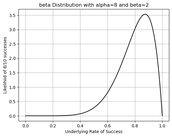
You are welcome to play around with the values here - what happens when you change \(\alpha\) (alpha) and \(\beta\) (beta)?
What does the Beta Distribution tell us?
Now how can we interpret this to find results? Lets think about what this function is telling us
The beta distribution gives us a probability density for each value of \(x\) between \(0.0\) and \(1.0\).
Can we plug in \(x\) values? Well, yes but what does this tell us?
alpha_val = 8
beta_val = 2

# What is the result if we just plug into the function?
# Does this give the chance of getting a 90\% underlying probability if we do 8/10 trials?
prob_density = beta.pdf(0.9, alpha_val, beta_val)
print(prob_density)3.4437376800000004Okay at the exact point \(x=0.9\) we see we have a function height of about 3.44%. Does this mean that there is exactly a 3.44% chance that if I get 8/10 success then I had 90% as my underlying probability? This is the same as asking if I randomly picked an underlying probability from between 0 and 1 with this distribution, would I get exactly 0.9 with a probability of 3.44%? NO THIS DOES NOT WORK
What is going on here:
- In the discrete, Binomial Distribution, case I could just plug in \(k=8\) and get the probability for that case. A big difference here is that there were only a discrete number of outcomes - think marbles in a bag. So if I was picking randomly there really would be a 19.37% chance of picking \(k=8\)
- In the continuous case, Beta Distribution, I cannot just plug in \(x=0.9\). Why not? If I was picking randomly from a bag of marbles in the continuous cases there would be an infinite number of marbles in there!! The chance of actually getting exactly \(x=0.9\) is zero - same as the probability of choosing exactly one unique marble from an infinite number.
- The continuous probability density function is more like a RATE (probability per probability) so to get the probability we need to integrate - or find the area under the curve.
The above calculation
\[AREA = BASE * HEIGHT = 0 * 3.4437376800000004 = 0\]
Okay, but if we can’t just plug in - this is this thing worthless? NO - what do we do when given a rate (density) and wanting to know the value (area under curve)?
Calculus to the rescue!
The beta distribution is a probability distribution. This means that the area under the whole curve must be equal to 1.0 or 100% (There is 100% chance that my underlying probability is between 0 and 100). To find a specific probability we need to find the area under the curve within a range. Here is some notation to support our discussion:
Assume that \(f(x,\alpha,\beta)\) is a beta distribution then:
\[\int_0^1 f(x,\alpha,\beta)\;dx = 1\]
If I wanted to know something like what is the probability that \(x\leq 0.9\)? I would have to integrate:
\[P(X\leq 0.9) = \int_0^{0.9} f(x,\alpha,\beta)\;dx \]
What if I wanted to know what is the probability that \(x\geq 0.9\)?
\[P(X\geq 0.9) = \int_{0.9}^{1} f(x,\alpha,\beta)\;dx = 1-\int_0^{0.9} f(x,\alpha,\beta)\;dx \]
Okay so we are throwing around some crazy notation here! What the are those numbers on the integral sign? In our discussion of integration we talked only about integrals that looked like this
\[\int f(x)\;dx = F(x) + c\]
this is called in indefinte integral. We wanted a family of functions that we could use for our analysis. But the whole idea is that the integral was the area under the curve. If instead I write
\[\int_a^b f(x)\;dx\]
this is putting limits of integration on my integral. This means we are only interested in adding up the area under the curve between the values of \(a\leq x \leq b\) and since this is an exact area that I can color in… the result is a number.
Plot \(P(X\leq 0.9)\)
alpha_val = 8
beta_val = 2
a = 0
b = 0.9

# Generate x values (range from 0 to 1)
x = np.linspace(0, 1, 100)
# Calculate the probability density function (PDF)
pdf = beta.pdf(x, alpha_val, beta_val)

plt.plot(x,pdf,'-k')

# Color in the area under the curve from 0 to 0.9
x_fill = np.linspace(a, b, 100)
pdf_fill = beta.pdf(x_fill, alpha_val, beta_val)
plt.fill_between(x_fill, pdf_fill, color='lightblue', alpha=0.7, label='Area up to 0.9')

plt.title(f'beta Distribution with alpha={alpha_val} and beta={beta_val}')
plt.xlabel('Underlying Rate of Success')
plt.ylabel(f'Likelihiid of {alpha_val}/{alpha_val+beta_val} successes')
plt.grid()
plt.show()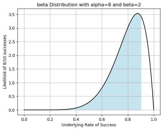
Plot \(P(X\leq 0.9)\)
alpha_val = 8
beta_val = 2
a = 0.9
b = 1

# Generate x values (range from 0 to 1)
x = np.linspace(0, 1, 100)
# Calculate the probability density function (PDF)
pdf = beta.pdf(x, alpha_val, beta_val)

plt.plot(x,pdf,'-k')

# Color in the area under the curve from 0 to 0.9
x_fill = np.linspace(a, b, 100)
pdf_fill = beta.pdf(x_fill, alpha_val, beta_val)
plt.fill_between(x_fill, pdf_fill, color='lightblue', alpha=0.7, label='Area up to 0.9')

plt.title(f'beta Distribution with alpha={alpha_val} and beta={beta_val}')
plt.xlabel('Underlying Rate of Success')
plt.ylabel(f'Likelihiid of {alpha_val}/{alpha_val+beta_val} successes')
plt.grid()
plt.show()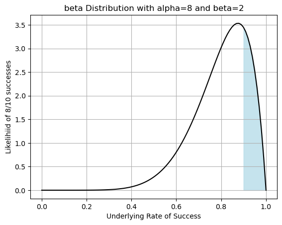
Cumulative Distribution Function
This area under the curve is represented by the cumulative distribution function (CDF) the whole job of this function is to add up the area under the curve between 0 and some value (adding up the probability densities). Here is the official definition:
Mathematically, it is defined as:
\[F(x; \alpha, \beta) = P(X \le x) = \int_0^x f(x,\alpha,\beta) dt\]
notice that it is always defined with the bottom limit being zero.
Luckily our scipy beta function already has this programmed for us!
alpha_val = 8
beta_val = 2
x_val = 0.9

# We use the beta.cdf() function to calculate the cumulative distribution
p = beta.cdf(x_val,alpha_val,beta_val)
print(p)0.7748409780000002Interpret the results
This means that there is a 77.48% chance that the underlying probability of success of our engine trials was less then 90% OR that there was a 1-77.48% = 22.52% chance that the underlying probability of success was greater than 90%.
So thinking back to our original experiment. The odds are not in our favor. There is a higher chance that the underlying success rate is lower than 90% and maybe we should cut our losses. But maybe our CFO has a bit of funding to send our way.
You try
Imagine that you are an engineer on this problem and you just finished doing more tests of the engine. You found that you had a total of 30 successes and 6 failures. Answer the following questions:
- What is your new marginal probability of success?
Binomial Distribution Questions
- What is the probability that you got exactly 30 successes in 36 trials if you had an underlying success rate of 90%?
- Plot the binomial distribution for these experiments.
- What is the probability that we had 30 or fewer successes?
- What is the probability that we had more than 30 successes?
beta Distribution Questions
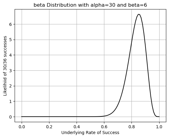
- Plot the beta distribution for this example, here you have 30 successes and 6 failures.
- Compare the shape of this beta distribution to the one we did before.
- What is the probability that our underlying success rate is 90% or better?
- What does this say about our doing more experiments - your opinion backed by math.
Challenge
- Calculate the probability that your underlying success rate is between 80% and 90%. HINT Use the cumulative distribution function in python and think about the areas under the curve and do some algebra to get the right area.
HERE IS JOANNA’S CODE - MAKE SURE YOU TRY ON YOUR OWN FIRST
Code
print("Joanna's Results")
print('------------------')

a=30
b=6
n = 36 # Number of Trials
p = 0.9 # Probability of Success
K = 30 # Focal number of successes

print(f'Prob of success: {a/(a+b)}')

engine_binom = []
k_vals = []
for k in range(n+1):
    k_vals.append(k)
    P = binom.pmf(k,n,p)
    engine_binom.append(P)
    if k==K:
        print(f'The probability of {k} successes in {n} experiments is P(X={k})={P}')

plt.bar(k_vals,engine_binom)
plt.title('A Binomial Distribuion - Engine Example')
for i, value in enumerate(engine_binom):
    plt.text(i, value, str(round(value,4)), ha='center', va='bottom',rotation=45) # Adjust vertical offset (+1) as needed

plt.xlabel(f'k outcomes in n={n} trials')
plt.ylabel('Probability')
plt.show()

start = 0
end = 30
print(f'The probability that we had fewer than 30 successes: {sum(engine_binom[start:end+1])}')

start = 31
end = 36
print(f'The probability that we had more than 30 successes: {sum(engine_binom[start:end+1])}')


# Generate x values (range from 0 to 1)
x = np.linspace(0, 1, 100)
# Calculate the probability density function (PDF)
pdf = beta.pdf(x, a, b)

plt.plot(x,pdf,'-k')
plt.title(f'beta Distribution with alpha={a} and beta={b}')
plt.xlabel('Underlying Rate of Success')
plt.ylabel(f'Likelihiid of {a}/{a+b} successes')
plt.grid()
plt.show()

x_val = 0.9
# We use the beta.cdf() function to calculate the cumulative distribution
p = beta.cdf(x_val,a,b)
print(f'The probability that my success rate is higher than 90\% is {1-p}')
Joanna's Results
------------------
Prob of success: 0.8333333333333334
The probability of 30 successes in 36 experiments is P(X=30)=0.08256915895919979
The probability that we had fewer than 30 successes: 0.14539730133503703
The probability that we had more than 30 successes: 0.8546026986649633
The probability that my success rate is higher than 90\% is 0.13163577484183697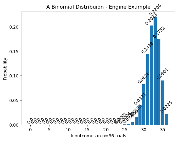
Code
print('CHALLENGE')
a=30
b=6
p1 = beta.cdf(0.9,a,b)
p2 = beta.cdf(0.8,a,b)
print(f'The probability that my success rate is between 80 and 90 is {p1-p2}')
CHALLENGE
The probability that my success rate is between 80 and 90 is 0.5962725311986752Extra - mathematical definition of the beta distribution
The beta probability density function (PDF) is given by:
\[f(x; \alpha, \beta) = \frac{x^{\alpha-1} (1-x)^{\beta-1}}{B(\alpha, \beta)}\]
where:
- \(0 \le x \le 1\).
- \(\alpha\) and \(\beta\) are parameters, with \(\alpha > 0\) and \(\beta > 0\).
- \(B(\alpha, \beta)\) is the beta function, which is a normalization constant that ensures the total probability integrates to 1. It is defined as:
\[B(\alpha, \beta) = \int_0^1 t^{\alpha-1} (1-t)^{\beta-1} dt = \frac{\Gamma(\alpha) \Gamma(\beta)}{\Gamma(\alpha + \beta)}\]
- \(\Gamma(z)\) is the gamma function, a generalization of the factorial function to complex numbers. For positive integers, \(\Gamma(n) = (n-1)!\).
The beta distribution can also be written as:
\[f(x; \alpha, \beta) = \frac{\Gamma(\alpha + \beta)}{\Gamma(\alpha) \Gamma(\beta)} x^{\alpha-1} (1-x)^{\beta-1}\]