# We will just go ahead and import all the useful packages first.
import numpy as np
import sympy as sp
import pandas as pd
import matplotlib.pyplot as plt
from mpl_toolkits.mplot3d import Axes3D

# Special Functions
from sklearn.metrics import r2_score, mean_squared_error

## NEW
from scipy.stats import binom, beta, norm

# Functions to deal with dates
import datetimeMath for Data Science
Introduction to Linear Algebra
Important Information
- Email: joanna_bieri@redlands.edu
- Office Hours take place in Duke 209 unless otherwise noted – Office Hours Schedule
Today’s Goals:
- What is Linear Algebra
- Vectors
- Addition, Magnitude, Scalar Multiplication, Subtraction
- K Nearest Neighbors - Machine Learning Classification
# Some helpful functions for visualizations today
def plot_vector(vector,origin=(0, 0), color='b', label=None, lims=True):
    """Plots a vector from the origin."""
    plt.quiver(origin[0], origin[1], vector[0], vector[1],
               angles='xy',
               scale_units='xy',
               scale=1,
               color=color,
               label=label,
               headwidth=3,
               headlength=4)
    if lims:
        plt.xlim(-1, vector[0]+1)
        plt.ylim(-1, vector[1]+1)
    plt.xlabel('x')
    plt.ylabel('y')
    plt.title('Vector Plot')
    plt.grid(True)

def vector_addition(v1, v2):
    """Adds two vectors and plots the result."""
    result = v1 + v2
    plot_vector(v1, color='b', label='v1')
    plot_vector(v2,origin=(v1[0],v1[1]), color='g', label='v2')
    plot_vector(result, color='r', label='v1 + v2')
    plt.legend()
    plt.title('Vector Addition')
    plt.grid(True)
    plt.show()
    return result

def vector_subtraction(v1, v2):
    """Subtracts v2 from v1 and plots the result."""
    result = v1 - v2
    plot_vector(v1, color='b', label='v1')
    plot_vector(v2, color='g', label='v2')
    plot_vector(result,origin=(v2[0],v2[1]), color='m', label='v1 - v2')
    plt.legend()
    plt.title('Vector Subtraction')
    plt.grid(True)
    # Autoscale the axes based on the vectors
    all_x = [0, v1[0], v2[0], v1[0] - v2[0]]
    all_y = [0, v1[1], v2[1], v1[1] - v2[1]]

    min_x = min(all_x) - 1  # Add a little buffer
    max_x = max(all_x) + 1
    min_y = min(all_y) - 1
    max_y = max(all_y) + 1

    plt.xlim(min_x, max_x)
    plt.ylim(min_y, max_y)
    plt.axhline(0, color='black', linewidth=0.5)
    plt.axvline(0, color='black', linewidth=0.5)
    plt.show()
    return result

def scalar_multiplication(vector, scalar):
    """Multiplies a vector by a scalar and plots the result."""
    result = vector * scalar
    plot_vector(vector, color='b', label='v')
    plot_vector(result, color='c', label=f'{scalar} * v')
    plt.legend()
    plt.title(f'Scalar Multiplication (Scalar = {scalar})')
    plt.grid(True)
    plt.axhline(0, color='black', linewidth=0.5)
    plt.axvline(0, color='black', linewidth=0.5)
    plt.show()
    return result

def magnitude_and_direction(vector):
    """Calculates and prints the magnitude and direction of a vector, and plots it."""
    magnitude = np.linalg.norm(vector)
    direction = np.arctan2(vector[1], vector[0])  # Returns angle in radians
    direction_degrees = np.degrees(direction)

    print(f"Magnitude: {magnitude}")
    print(f"Direction: {direction_degrees} degrees")
    plot_vector(vector, color='k', label='Vector')
    plt.legend()
    plt.title('Magnitude and Direction')
    plt.grid(True)
    plt.axhline(0, color='black', linewidth=0.5)
    plt.axvline(0, color='black', linewidth=0.5)
    plt.show()
    return magnitude, direction_degrees
Linear Algebra
Linear algebra gives us a way to study linear systems. In my opinion Linear Algebra is one of the most important mathematical topics you can study to truly understand modern computation, data science, and machine learning. It is a fundamental tool behind the “black box” of many algorithms used in data science.
There are some scary terms used when talking about linear algebra: Vector, Matrix, Tensor, Eigenvalue, Inverse, Span, Basis, etc. I hope that by the end of this course these ideas feel more comfortable to you.
What is a Vector.
In the simplest words a vector is just an arrow in space with a specific direction and length. In two dimensions it is given by two numbers
\[\vec{v} = \begin{bmatrix} a \\ b \end{bmatrix}\]
\(a\) and \(b\) are just numbers that tell me how far to go in each direction. Vectors exist independently of a coordinate system, although we imagine them with their tail at \((0,0)\) and their point at \((a,b)\)
Example:
\[\vec{v} = \begin{bmatrix} 3 \\ 2 \end{bmatrix}\]
# A vector as a list
v = [3,2]
plot_vector(v)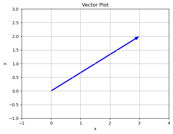
Here we can see that from \((0,0)\) we go three steps in the \(x\) direction and two steps in the \(y\) direction.
There are other ways to input a vector in Python:
- Use Numpy if you want to do numerical calculations
- Use Sympy if you want symbolic results.
# A vector in Numpy
v = np.array([3,2])
print(v)
[3 2]# A vector in Sympy
v = sp.Matrix([3,2])
v\(\displaystyle \left[\begin{matrix}3\\2\end{matrix}\right]\)
You Try
Here are three more examples of vectors. First draw the vector by hand, then compare what what you get by using the code below.
\[\vec{v} = \begin{bmatrix} 3 \\ 4 \end{bmatrix}\]
\[\vec{v} = \begin{bmatrix} -3 \\ 2 \end{bmatrix}\]
\[\vec{v} = \begin{bmatrix} -4 \\ -4 \end{bmatrix}\]
# Enter your vector as a list
v = [3,2]

# Run the cell to plot it
plot_vector(v)
Why are Vectors Useful?
A vector can represent many different things:
- Navigation systems (GPS).
- Robotics (path planning).
- Physics (forces, velocities).
- Game development.
- Classification and Distances.
- Abstract systems.
For example, say you have information about the square footage of a home and it’s sales price. We can put this information into a vector so that we can more easily do operations on it.
- Square footage = 1500
- Price = 450000
- \[\vec{v} = \begin{bmatrix} 1500 \\ 450000 \end{bmatrix}\]
In fact the inputs into machine learning models are represented as vectors.
Higher Dimensions
The beautiful thing about vectors is that you can develop intuition about them in just 2-dimensions but the ideas work no matter how many dimensions you have. We can still visualize three dimensions as an arrow in three dimensional space:
\[\vec{v} = \begin{bmatrix} 4 \\ 1 \\ 2 \end{bmatrix}\]
This vector starts at \((0,0)\) then you go 4 steps in the \(x\) direction, \(1\) step in the \(y\) direction and \(2\) steps in the \(z\) direction.
In many machine learning examples you will have multiple input features - columns in your data that you think help you predict something important. You will often put these features into a vector for each observation.
Adding Vectors
Adding vectors allows us to combine the movements of two vectors into a single instruction. Let look at an example:
\[\vec{v} = \begin{bmatrix} 3 \\ 2 \end{bmatrix}\]
\[\vec{w} = \begin{bmatrix} 2 \\ -1 \end{bmatrix}\]
When you add vectors you add their components
\[\vec{v}+\vec{w} = \begin{bmatrix} 3 \\ 2 \end{bmatrix} + \begin{bmatrix} 2 \\ -1 \end{bmatrix} = \begin{bmatrix} 3 + 2 \\ 2 + (-1) \end{bmatrix}= \begin{bmatrix} 5 \\ 1 \end{bmatrix} \]
v = np.array([3,2])
w = np.array([2,-1])

v_plus_w = vector_addition(v,w)
print(v_plus_w)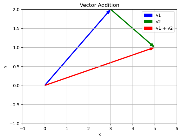
[5 1]We can think about what this addition means by the fact that we can get to the final location either by following the blue and then the green vector OR by just following the red vector. The addition is combining these steps into a single instruction.
Also, we could have done this in any order! We get the same result
\[ \vec{v}+\vec{w} = \vec{w}+\vec{v}\]
v = np.array([3,2])
w = np.array([2,-1])

w_plus_v = vector_addition(w,v)
print(v_plus_w)
[5 1]# In numpy
v = np.array([3,2])
w = np.array([2,-1])
v+warray([5, 1])You Try
Consider the vectors: \[\vec{v} = \begin{bmatrix} 3 \\ 4 \end{bmatrix}\] \[\vec{u} = \begin{bmatrix} -3 \\ 2 \end{bmatrix}\] \[\vec{w} = \begin{bmatrix} -4 \\ -4 \end{bmatrix}\]
Find the following sums. First do the calculation and drawing by hand then use the code below to check your answer.
- \(\vec{v}+\vec{u}\)
- \(\vec{u}+\vec{v}\)
- \(\vec{v}+\vec{u}+\vec{w}\)
# Enter your vectors here:
v = np.array([3,2])
w = np.array([2,-1])

w_plus_v = vector_addition(w,v)
print(v_plus_w)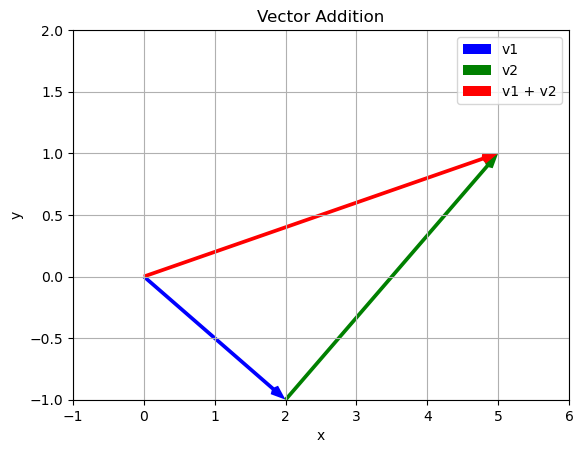
[5 1]Magnitude and Direction of a Vector
The magnitude of a vector is a measure of it’s length and it’s direction is a measure of the angle between it and the \(x\)-axis. To get these values we can use trigonometry!
Magnitude - use Pythagorean Theorem
We know the bottom side is 3 units and the right side is 2 units so the hypotenuse - or the length is
\[ ||\vec{v}|| = \sqrt{3^2+2^2} = \sqrt{9+4} = \sqrt{13}\]
We can also use the python code
np.linalg.norm()Angle - use Tangent
We know that in a right triangle the tangent of the angle is the opposite side over the adjacent side:
\[\tan(\theta) = opp/adj\]
so for our vector
\[\tan(\theta) = \frac{2}{3}\]
and solving for the angle
\[\theta = \arctan\left(\frac{2}{3}\right) = \tan^{-1}\left(\frac{2}{3}\right)\]
v = np.array([3,2])

magnitude_and_direction(v)
Magnitude: 3.605551275463989
Direction: 33.690067525979785 degrees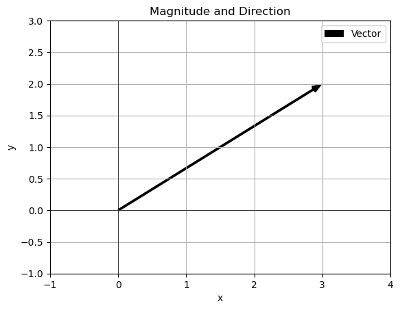
You Try
Consider the vectors: \[\vec{v} = \begin{bmatrix} 3 \\ 4 \end{bmatrix}\] \[\vec{u} = \begin{bmatrix} -3 \\ 2 \end{bmatrix}\] \[\vec{w} = \begin{bmatrix} -4 \\ -4 \end{bmatrix}\]
- Find the magnitude of each vector write out the formula by hand. You can use python to check your work, see the code below, but you should draw the vector and write out the Pythagorean formula.
# Finding the magnitude of v=[3,2]
v = np.array([3,2])

np.linalg.norm(v)3.605551275463989Scaling Vectors
Now that we can find the magnitude of a vector, we might want to shrink or extend the vector, without changing the direction. This is called scaling - or scalar multiplication
What is a scalar, this is just a number like we are use to. It has only a single value.
Example
\[\vec{v} = \begin{bmatrix} 3 \\ 2 \end{bmatrix}\]
then
\[2\vec{v} = 2\begin{bmatrix} 3 \\ 2 \end{bmatrix}= \begin{bmatrix} 2*3 \\ 2*2 \end{bmatrix}= \begin{bmatrix} 6 \\ 4 \end{bmatrix}\]
In this case we multiply each component of the vector by the scalar.
v = np.array([3,2])
s = 2
scalar_multiplication(v,s)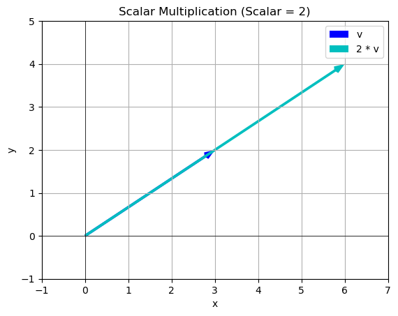
array([6, 4])You Try
Consider the vectors: \[\vec{v} = \begin{bmatrix} 3 \\ 4 \end{bmatrix}\] \[\vec{u} = \begin{bmatrix} -3 \\ 2 \end{bmatrix}\] \[\vec{w} = \begin{bmatrix} -4 \\ -4 \end{bmatrix}\]
Find \(4\vec{v}\)
Find \(-1\vec{w}\)
Find \(\frac{1}{2}\vec{u}\)
Do the vectors change direction in any of these cases?
For each of these do the calculation by hand, draw the picture, and then check your results using the code below.
# Enter your vector
v = np.array([3,2])
# Enter your scalar
s = 2
scalar_multiplication(v,s)
array([6, 4])K-nearest Neighbors Classifier
Here is a real world example where vectors are used in Data Science and Machine Learning!
The K-Nearest Neighbors (K-NN) algorithm is a popular Machine Learning algorithm used mostly for solving classification problems. It uses a set of discrete steps to decide how to classify a test point based on existing data.
Given a new data point
- Choose how many neighbors you want to use (\(K\))
- Calculate the distance between the new data point and all other points in the data set. (vector magnitude).
- Find the \(K\) nearest neighbors to the new data point based in the distances.
- Assign the new data entry to the class that is in the majority of nearest neighbors. If there is a tie - come up with tie breaker rule! Often we increase or decrease K.
Data
Let’s say you gather the following data about a group of people
file_location = 'https://joannabieri.com/mathdatascience/data/ice_cream_classifier.csv'
DF = pd.read_csv(file_location)
DF| Sweetness | Fruitiness | Flavor | |
|---|---|---|---|
| 0 | 2 | 3 | Vanilla |
| 1 | 8 | 9 | Strawberry |
| 2 | 9 | 2 | Chocolate |
| 3 | 7 | 8 | Strawberry |
| 4 | 3 | 7 | Vanilla |
| 5 | 5 | 5 | Vanilla |
| 6 | 6 | 7 | Strawberry |
| 7 | 8 | 3 | Chocolate |
| 8 | 4 | 4 | Vanilla |
| 9 | 7 | 4 | Chocolate |
# Separate data by flavor
vanilla_data = DF[DF['Flavor'] == 'Vanilla']
strawberry_data = DF[DF['Flavor'] == 'Strawberry']
chocolate_data = DF[DF['Flavor'] == 'Chocolate']

# Plotting
plt.figure(figsize=(8, 6))
plt.scatter(vanilla_data['Sweetness'], vanilla_data['Fruitiness'], color='lightblue', label="Vanilla")
plt.scatter(strawberry_data['Sweetness'], strawberry_data['Fruitiness'], color='red', label="Strawberry")
plt.scatter(chocolate_data['Sweetness'], chocolate_data['Fruitiness'], color='brown', label="Chocolate")

plt.xlabel("Sweetness")
plt.ylabel("Fruitiness")
plt.title("Ice Cream Flavors")
plt.legend()
plt.grid(True)
plt.xlim(0,10)
plt.ylim(0,10)
plt.show()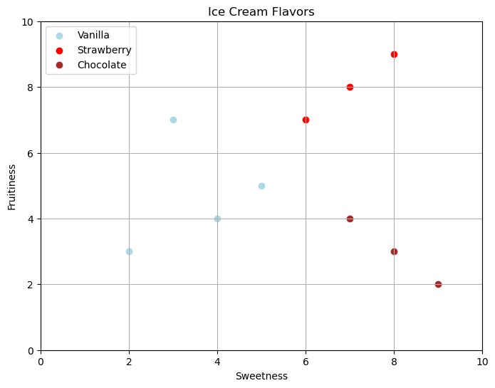
Now imagine that you have a new person that who has the data
query_vector = np.array([6, 6])\[\vec{q} = \begin{bmatrix} Sweetness \\ Fruitiness \end{bmatrix}=\begin{bmatrix} 6 \\ 6 \end{bmatrix}\]
query_vector = np.array([6, 6])

# Separate data by flavor
vanilla_data = DF[DF['Flavor'] == 'Vanilla']
strawberry_data = DF[DF['Flavor'] == 'Strawberry']
chocolate_data = DF[DF['Flavor'] == 'Chocolate']

# Plotting
plt.figure(figsize=(8, 6))
plt.scatter(vanilla_data['Sweetness'], vanilla_data['Fruitiness'], color='lightblue', label="Vanilla")
plt.scatter(strawberry_data['Sweetness'], strawberry_data['Fruitiness'], color='red', label="Strawberry")
plt.scatter(chocolate_data['Sweetness'], chocolate_data['Fruitiness'], color='brown', label="Chocolate")
plt.scatter(query_vector[0], query_vector[1], color='red', marker='*', s=200, label='Query Person')

plt.xlabel("Sweetness")
plt.ylabel("Fruitiness")
plt.title("Ice Cream Flavors")
plt.legend()
plt.grid(True)
plt.xlim(0,10)
plt.ylim(0,10)
plt.show()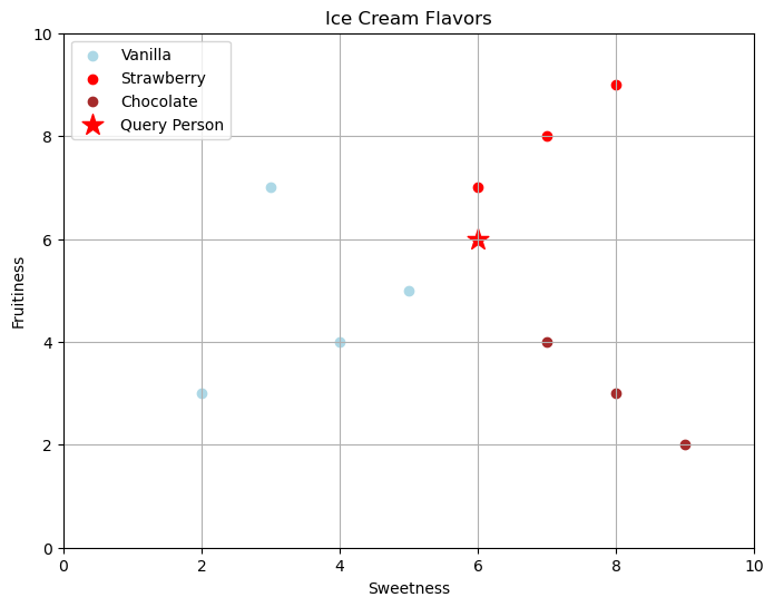
- We will choose \(K=4\) to start, but this is just a choice!
- Calculate the distance between the new data point and all other points in the data set. (vector magnitude).
Now in this case the distance between two points is the magnitude of the vector between the two arrow points. To see how far apart my query vector and another data vector are we can subtract them and then find the magnitude
\[\vec{q} = \begin{bmatrix} 6 \\ 6 \end{bmatrix}\]
\[\vec{d_1} = \begin{bmatrix} 2 \\ 3 \end{bmatrix}\]
\[\vec{q}-\vec{d_1} = \vec{q}+(-\vec{d_1}) = \begin{bmatrix} 6 \\ 6 \end{bmatrix}+\begin{bmatrix} -2 \\ -3 \end{bmatrix}=\begin{bmatrix} 4 \\ 3 \end{bmatrix}\]
then find the magnitude
q=np.array([6,6])
d1 = np.array([2,3])

# Get the subtraction
vec = vector_subtraction(q,d1)

# Find the norm
np.linalg.norm(vec)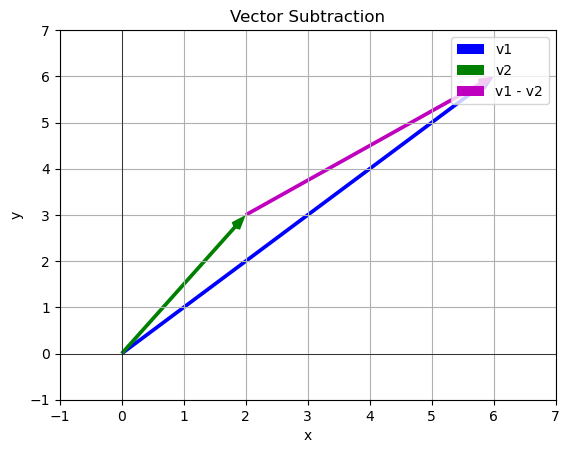
5.0# Now do this for all the points:
data = DF[['Sweetness','Fruitiness']].values
labels = list(DF['Flavor'])
distances = []
for i, vector in enumerate(data):
distance = np.linalg.norm(query_vector-vector)
distances.append((distance, labels[i]))
distances[(5.0, 'Vanilla'),
(3.605551275463989, 'Strawberry'),
(5.0, 'Chocolate'),
(2.23606797749979, 'Strawberry'),
(3.1622776601683795, 'Vanilla'),
(1.4142135623730951, 'Vanilla'),
(1.0, 'Strawberry'),
(3.605551275463989, 'Chocolate'),
(2.8284271247461903, 'Vanilla'),
(2.23606797749979, 'Chocolate')]- Get the K nearest points
K=4
distances.sort()
distances[:K]
[(1.0, 'Strawberry'),
(1.4142135623730951, 'Vanilla'),
(2.23606797749979, 'Chocolate'),
(2.23606797749979, 'Strawberry')]It looks like we should suggest that this person tries Strawberry Ice Cream!
KNN in Python!
Python Sklearn has a KNN function!
from sklearn.neighbors import KNeighborsClassifier

# First we train our ML model
# NOTE - we are skipping some important ideas from ML
#        like test train split and checking accuracy
#        this code is just intended to demonstrate how vectors are used.

# These are the vector inputs
data = DF[['Sweetness','Fruitiness']].values
# These are the labels - classifications
labels = list(DF['Flavor'])

# Build the classifier model
knn_4 = KNeighborsClassifier(n_neighbors=4) # Update the number of neighbors
knn_4.fit(data,labels)KNeighborsClassifier(n_neighbors=4)In a Jupyter environment, please rerun this cell to show the HTML representation or trust the notebook.
On GitHub, the HTML representation is unable to render, please try loading this page with nbviewer.org.
KNeighborsClassifier(n_neighbors=4)
# Now try to make a prediction

query_vector = np.array([6,6])

# Run a new query through the model
query = query_vector.reshape(1, -1)
suggestion = knn_4.predict(query)
print(suggestion)['Strawberry']You can see that we got the prediction we expected! You can play around with this code and see what happens for different queries.
You Try
Consider the video game data below. Imagine you survey 10 video game enthusiast and ask them to say what kind of game they prefer and rank the amount of action and story content they like to have in a game. Now we are going to use this data to build a system that will recommend a game type to a new player based on their scores for action and story.
New player (query) vector:
\[\vec{q} = \begin{bmatrix} Action \\ Story \end{bmatrix}=\begin{bmatrix} 6 \\ 4 \end{bmatrix}\]
Please do the following:
- Choose one of the data vectors and write it down in vector form.
- Find the vector that is difference between to two \(\vec{q}-\vec{data}\)
- Plot these vectors using the code below.
- Find the distance between the two - magnitude of the difference.
- Using Sklearn KNeighborsClassifier, build a KNN with K=3.
- Predict the type of game your new player would want to play.
file_location = 'https://joannabieri.com/mathdatascience/data/videogames.csv'
DF_vg = pd.read_csv(file_location)
DF_vg| Amt Action | Amt Story | Type | |
|---|---|---|---|
| 0 | 3 | 9 | RPG |
| 1 | 9 | 4 | Action |
| 2 | 5 | 8 | RPG |
| 3 | 10 | 2 | Action |
| 4 | 6 | 7 | RPG |
| 5 | 2 | 6 | RPG |
| 6 | 9 | 3 | Action |
| 7 | 4 | 7 | RPG |
| 8 | 8 | 5 | Action |
| 9 | 7 | 3 | Action |
# Separate data by Type
RPG_data = DF_vg[DF_vg['Type'] == 'RPG']
Action_data = DF_vg[DF_vg['Type'] == 'Action']


# Plotting
plt.figure(figsize=(8, 6))
plt.scatter(RPG_data['Amt Action'], RPG_data['Amt Story'], color='lightblue', label="RPG")
plt.scatter(Action_data['Amt Action'], Action_data['Amt Story'], color='red', label="Action")

plt.xlabel("Action")
plt.ylabel("Story")
plt.title("Video Games")
plt.legend()
plt.grid(True)
plt.xlim(0,12)
plt.ylim(0,12)
plt.show()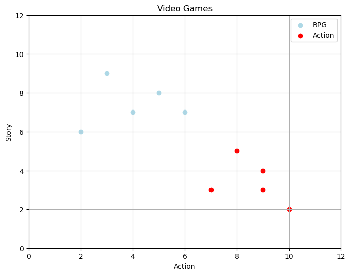
# q = #Query
# d1 = #data point

# # Get the subtraction
# vec = vector_subtraction(q,d1)

# # Find the norm
# np.linalg.norm(vec)
# # These are the vector inputs
# data = DF[['Amt Action', 'Amt Story']].values
# # These are the labels - classifications
# labels = list(DF['Type'])
# # Build the classifier model
# knn = KNeighborsClassifier(n_neighbors=4) # Update the number of neighbors
# knn.fit(data,label)# # This is the data you want to classify
# query_vector = np.array([6,6])
# # Run a new query through the model
# query = query_vector.reshape(1, -1)
# suggestion = knn.predict(query)
# print(suggestion)