import numpy as np
import sympy as spMath for Data Science
Start Calculating in Python - More Math Fundamentals
Important Information
- Email: joanna_bieri@redlands.edu
- Office Hours take place in Duke 209 unless otherwise noted – Office Hours Schedule
Todays Goals:
- Continue using Python as a calculator.
- What do errors look like?
- More math review.
Sympy and Numpy
Numpy is ….
Sympy is ….
Get out a piece of paper and do the calculations by hand as we go through the python code!
What do errors look like:
a = sp.Rational(3/2)
np.sin(a)
TypeError: loop of ufunc does not support argument 0 of type Rational which has no callable sin methoda = sp.rational(3,2)AttributeError: module 'sympy' has no attribute 'rational'a^3TypeError: unsupported operand type(s) for ^: 'Rational' and 'int'c**3NameError: name 'c' is not definedA bit more practice Algebra, Logs, and Exponents
Here are some more practice problems. You should:
Do the problem by hand.
Write python code to do the problems.
Compare your answers.
Add the fractions: \[ \frac{x}{2}+\frac{x}{3}+\frac{x}{4}\]
Solve for \(x\): \[3x+2-5=4^2\]
Simplify the expression: \[2^33-3\]
Simplify the expression: \[\ln(e^{\frac{4-2}{3^3}})\]
Solve for \(x\): \[\log_4(x)=2\]
# What does this do?
x = sp.symbols('x')
Example - Solve for x
\[ e^{x^2-4}=1 \]
# How would we solve for x?

# Enter the expression with everything solved to one side:
my_expr = sp.exp(x**2-4)-1
my_expr
\(\displaystyle e^{x^{2} - 4} - 1\)
# Use sp.solve to solve my_expr=0 for x
sp.solve(my_expr,x)
[-2, 2]Example - Solve for x - weird answer
\[ e^{x^2-4}=-1 \]
my_expr = sp.exp(x**2-4)+1
my_expr
\(\displaystyle e^{x^{2} - 4} + 1\)
sp.solve(my_expr,x)[-sqrt(4 + I*pi), sqrt(4 + I*pi)]What happened here? Why the weird output?
Geometry and Trigonometry
Some of you have have a lot of experience with trigonometry and some might have just barely seen it. In many cases solving problems in this area is about correctly applying formulas and then doing some algebra and arithmetic to solve.
1. What is the area of a circle with radius \(r=10\) meters.
Well first we have to remember the formula \(A=\pi r^2\) and then we can plug in!
A = np.pi*10**2
A314.1592653589793# Or we could enter it as a formula in sympy - so we can use it again and again!
rad = 10
r = sp.symbols('r')
A = sp.pi*r**2
A.subs(r,rad)\(\displaystyle 100 \pi\)
2. If a right triangle has sides \(a=10\) and \(b=12\) then what is the length of the hypotenuse?
Here we have to remember the Pythagoren theorem: \(a^2 + b^2 = c^2\), where \(a\) and \(b\) are the sides and \(c\) is the hypotenuse.
c = np.sqrt(10**2+12**2)
c15.620499351813308# Or we could enter it as a formula in sympy - so we can use it again and again!
a = 10
b = 12
c = sp.symbols('c')
my_expr = a**2+b**2-c**2
sp.solve(my_expr,c)[-2*sqrt(61), 2*sqrt(61)]2*np.sqrt(61)15.6204993518133083. For what values of \(x\) does the function \(y=\sin(x)\) have zeros?
There are a few ways to approach zeros of a function. I usually start with a graph!
x = sp.symbols('x')
f = sp.sin(x)
plt = sp.plot(f)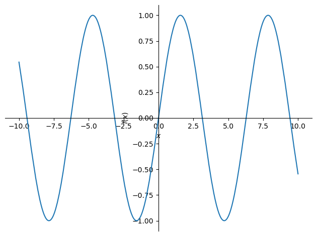
This tells me there are lots of zeros. Zeros are where the function crosses the \(x\)-axis!
What are the values of the zeros?
sp.solve(f,x)[0, pi]Solving Systems of TWO Equations
- Solve for \(x\) and \(y\): \[4x-y=12\] \[x+3y=1\]
There are actually many ways to think about solving problems like this!
- Solve EQ1 for y and then sub into EQ2…
- Stack the equations and simplify all at once - subtracting one equation from the next…
- Put the equations in Matrix form and solve…
Using sp.solve
x,y = sp.symbols('x,y')

eq1 = 4*x-y-12
eq2 = x+3*y-1

sp.solve([eq1, eq2], [x, y])
{x: 37/13, y: -8/13}If you wanted to see all the steps you could!
# Solve equation 1 for x in terms of y
sp.solve(eq1,x)
[y/4 + 3]# Sub the x solution into equation 2 and solve for y
xeqn = y/4+3
eq2 = xeqn+3*y-1
sp.solve(eq2,y)[-8/13]# Save the y value
yval = sp.Rational(-8,13)
yval\(\displaystyle - \frac{8}{13}\)
# Substitute the y value back into the x equation.
xval = yval/4+3
xval
\(\displaystyle \frac{37}{13}\)
What does it mean to solve a linear system?
We are looking for a point \((x*,y*)\) that is on BOTH lines:
\[ y = 4x-12 \] \[ y = \frac{1-x}{3} \]
We solve this to see that \((37/13, -8/13)\) is this point.
# What are these in decimal form
(37/13, -8/13)
(2.8461538461538463, -0.6153846153846154)# Enter the equations:
y_eq1 = 4*x-12
y_eq2 = (1-x)/3# Look at the plot
plt = sp.plot(y_eq1,y_eq2)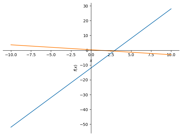
Solve the following linear systems and then plot the solution.
\[7x+2y=3\] \[4x+3y=11\]
\[\frac{x}{2}-\frac{y}{5}=-4\] \[3x+\frac{y}{2}=-7\]
First figure out the system of equations and then solve.
You run an accounting business that specializes in auditing (verifying accounting records). One of your auditors is working on the payroll records for a company with 75 employees. Some are part-time and some are full-time. After working for three days, your auditor tells you that the audit is completed for half of the full-time employees, but there are still 50 employee records to audit. Find out how many of the employees are full time and how many are part-time.
A financial planner wants to invest \$8000, some in stocks earning 15% annually and the rest in bonds earning 6% annually. How much should be invested at each rate to get a return of $930 annually from the two investments?
Factoring Polynomials
\[2x+12x^3\]
Factoring is basically undoing distribution. You are trying to break one polynomial apart into multiple polynomials. Sympy can help!
x = sp.symbols('x')
my_expr = 2*x+12*x**3
my_expr
\(\displaystyle 12 x^{3} + 2 x\)
sp.factor(my_expr)\(\displaystyle 2 x \left(6 x^{2} + 1\right)\)
Notice here that if we distribute \(2x\) into the polynomial \((6x^2+1)\) then we would get
\[ 12x^3 + 2x \]
which is the expression we started with!
Factor the following expressions
- \[x^2+9x\]
- \[x^2+9x-1\]
Solve the following expressions using factoring
- \[x^2-16=0\]
- \[x^2+9x-1=0\]
Expanding Polynomials
Sometimes we want to take a compact expression and expand it out to see what all of the terms are. This is like undoing the factoring.
x = sp.symbols('x')
my_expr = 2*x*(6*x**2+1)
my_expr
\(\displaystyle 2 x \left(6 x^{2} + 1\right)\)
sp.expand(my_expr)\(\displaystyle 12 x^{3} + 2 x\)
Expand the following expressions.
- \[ (x+4)^2 \]
- \[ x(x-3)(x+2) \]
remember if you are doing these by hand you have to FOIL the polynomials together!
Quadratic Formula - for those pesky polynomials that you can’t easily factor!
The quadratic formula works for any quadratic equation where you are solving for \(x\):
\[ ax^2+bx+c = 0 \]
here \(a\), \(b\), and \(c\) are just numbers. You can plug them into the formaula to find \(x\)
\[ x = \frac{-b \pm \sqrt{b^2-4ac}}{2a} \]
When you see strange outputs from the sp.solve() method you are probably running into the quadratic formula.
x = sp.symbols('x')
my_expr = x**2+9*x+6
my_expr
\(\displaystyle x^{2} + 9 x + 6\)
sp.solve(my_expr,x)[-9/2 - sqrt(57)/2, -9/2 + sqrt(57)/2]x = sp.symbols('x')
my_expr = x**2+3*x+6
my_expr\(\displaystyle x^{2} + 3 x + 6\)
sp.solve(my_expr,x)[-3/2 - sqrt(15)*I/2, -3/2 + sqrt(15)*I/2]