import numpy as np
import sympy as spMath for Data Science
Number Theory and Data Science
Important Information
- Email: joanna_bieri@redlands.edu
- Office Hours take place in Duke 209 unless otherwise noted – Office Hours Schedule
Today’s Goals:
- Define different types of numbers,variables and data
- How does basic math and number types apply to Data Science?
Important Types of Numbers
Natural Numbers 1,2,3….
Whole Numbers 0,1,2,3…
Integers …-3,-2,-1,0,1,2,3…
Rational Numbers Numbers that can be expressed fractions. Remember that \(3=\frac{3}{1}\) so this contains all the integers.
Irrational Numbers Decimal Numbers that cannot be expressed as fractions. They have an infinite number of decimal places. For example the number \(\pi\).
Real Numbers All rational and irrational numbers
Complex and Imaginary Numbers Numbers that contain the square root of negative 1. We express this as \(i=\sqrt{-1}\). These happen mathematically a lot!
Important types of Python Variables
int these are integers - no decimal
float these are rational or irrational numbers (within rounding). A computer can’t keep an infinite number of decimal places so there is rounding going on. Typically python will save 15-17 decimal digits of precision.
string these are words - anything with quotes around it.
Important types of Data Science Variables
Numerical - this is data represented by numbers
Categorical - this is data represented by strings
a = 1
b = 0.5
c = 'hello'
d = np.pitype(a)inttype(b)floattype(c)strtype(d)floatWhy does the number type (Number Theory) even matter?
Data is Messy!
When you are working with data a big part of your job will be cleaning data and deciding what types of numbers/variables should be allowed in the data. Here is an example of a messy data set about movies. It has 9999 observations (movies) listed and lots of information about those movies.
import pandas as pd

file_location = 'https://joannabieri.com/mathdatascience/data/movies.csv'
DF = pd.read_csv(file_location)

DF.head(10)| MOVIES | YEAR | GENRE | RATING | ONE-LINE | STARS | VOTES | RunTime | Gross | |
|---|---|---|---|---|---|---|---|---|---|
| 0 | Blood Red Sky | (2021) | \nAction, Horror, Thriller | 6.1 | \nA woman with a mysterious illness is forced ... | \n Director:\nPeter Thorwarth\n| \n Star... | 21,062 | 121.0 | NaN |
| 1 | Masters of the Universe: Revelation | (2021– ) | \nAnimation, Action, Adventure | 5.0 | \nThe war for Eternia begins again in what may... | \n \n Stars:\nChris Wood, \nSara... | 17,870 | 25.0 | NaN |
| 2 | The Walking Dead | (2010–2022) | \nDrama, Horror, Thriller | 8.2 | \nSheriff Deputy Rick Grimes wakes up from a c... | \n \n Stars:\nAndrew Lincoln, \n... | 885,805 | 44.0 | NaN |
| 3 | Rick and Morty | (2013– ) | \nAnimation, Adventure, Comedy | 9.2 | \nAn animated series that follows the exploits... | \n \n Stars:\nJustin Roiland, \n... | 414,849 | 23.0 | NaN |
| 4 | Army of Thieves | (2021) | \nAction, Crime, Horror | NaN | \nA prequel, set before the events of Army of ... | \n Director:\nMatthias Schweighöfer\n| \n ... | NaN | NaN | NaN |
| 5 | Outer Banks | (2020– ) | \nAction, Crime, Drama | 7.6 | \nA group of teenagers from the wrong side of ... | \n \n Stars:\nChase Stokes, \nMa... | 25,858 | 50.0 | NaN |
| 6 | The Last Letter from Your Lover | (2021) | \nDrama, Romance | 6.8 | \nA pair of interwoven stories set in the past... | \n Director:\nAugustine Frizzell\n| \n S... | 5,283 | 110.0 | NaN |
| 7 | Dexter | (2006–2013) | \nCrime, Drama, Mystery | 8.6 | \nBy day, mild-mannered Dexter is a blood-spat... | \n \n Stars:\nMichael C. Hall, \... | 665,387 | 53.0 | NaN |
| 8 | Never Have I Ever | (2020– ) | \nComedy | 7.9 | \nThe complicated life of a modern-day first g... | \n \n Stars:\nMaitreyi Ramakrish... | 34,530 | 30.0 | NaN |
| 9 | Virgin River | (2019– ) | \nDrama, Romance | 7.4 | \nSeeking a fresh start, nurse practitioner Me... | \n \n Stars:\nAlexandra Breckenr... | 27,279 | 44.0 | NaN |
# Look at just one row
display(DF.iloc[0])
MOVIES Blood Red Sky
YEAR (2021)
GENRE \nAction, Horror, Thriller
RATING 6.1
ONE-LINE \nA woman with a mysterious illness is forced ...
STARS \n Director:\nPeter Thorwarth\n| \n Star...
VOTES 21,062
RunTime 121.0
Gross NaN
Name: 0, dtype: objectWhat kind of numbers do we expect? What kind of variables are we getting? What does NaN mean?
- MOVIES – string or words
- YEAR – should be a number or integer
- GENRE – string or words
- RATING – should be a number or rational/float
- ONE-LINE – string or words
- STARS – string or words
- VOTES – should be a number or integer
- RunTime – should be a number - maybe integer maybe float?
- Gross – NaN means not a number - either infinity or no data was given
Some of the data is not the right format!!!!
display(DF['YEAR'].iloc[0])'(2021)'display(type(DF['YEAR'].iloc[0]))strThe data in the year column is a string not an integer. Can we just turn them all into integers? Not really! Some of the data represents a range of years!
Always keep track of what type of data you might be interacting with!
Feature Engineering
In data science we often do something called feature engineering this means taking given data and creating new data with it. Sometimes it is as simple as multiplying or adding to pieces of data. Sometimes it is much more complicated.
Here is an example data set where all of the variables have been encoded in some way. It describes the number of bikes that were rented in Washington DC. It gives information about the weather, and day of the week. For example
- season : season (1:spring, 2:summer, 3:fall, 4:winter)
- yr : year (0: 2011, 1:2012)
- mnth : month ( 1 to 12)
- hr : hour (0 to 23)
More complicated is how they “normalized” the temperatures.
- temp : Normalized temperature in Celsius. The values are divided to 41 (max)
- atemp: Normalized feeling temperature in Celsius. The values are divided to 50 (max)
- hum: Normalized humidity. The values are divided to 100 (max)
- windspeed: Normalized wind speed. The values are divided to 67 (max)
file_location = 'https://joannabieri.com/mathdatascience/data/bikeshare-day.csv'
DF = pd.read_csv(file_location)
DF.head(10)| instant | dteday | season | yr | mnth | holiday | weekday | workingday | weathersit | temp | atemp | hum | windspeed | casual | registered | cnt | |
|---|---|---|---|---|---|---|---|---|---|---|---|---|---|---|---|---|
| 0 | 1 | 2011-01-01 | 1 | 0 | 1 | 0 | 6 | 0 | 2 | 0.344167 | 0.363625 | 0.805833 | 0.160446 | 331 | 654 | 985 |
| 1 | 2 | 2011-01-02 | 1 | 0 | 1 | 0 | 0 | 0 | 2 | 0.363478 | 0.353739 | 0.696087 | 0.248539 | 131 | 670 | 801 |
| 2 | 3 | 2011-01-03 | 1 | 0 | 1 | 0 | 1 | 1 | 1 | 0.196364 | 0.189405 | 0.437273 | 0.248309 | 120 | 1229 | 1349 |
| 3 | 4 | 2011-01-04 | 1 | 0 | 1 | 0 | 2 | 1 | 1 | 0.200000 | 0.212122 | 0.590435 | 0.160296 | 108 | 1454 | 1562 |
| 4 | 5 | 2011-01-05 | 1 | 0 | 1 | 0 | 3 | 1 | 1 | 0.226957 | 0.229270 | 0.436957 | 0.186900 | 82 | 1518 | 1600 |
| 5 | 6 | 2011-01-06 | 1 | 0 | 1 | 0 | 4 | 1 | 1 | 0.204348 | 0.233209 | 0.518261 | 0.089565 | 88 | 1518 | 1606 |
| 6 | 7 | 2011-01-07 | 1 | 0 | 1 | 0 | 5 | 1 | 2 | 0.196522 | 0.208839 | 0.498696 | 0.168726 | 148 | 1362 | 1510 |
| 7 | 8 | 2011-01-08 | 1 | 0 | 1 | 0 | 6 | 0 | 2 | 0.165000 | 0.162254 | 0.535833 | 0.266804 | 68 | 891 | 959 |
| 8 | 9 | 2011-01-09 | 1 | 0 | 1 | 0 | 0 | 0 | 1 | 0.138333 | 0.116175 | 0.434167 | 0.361950 | 54 | 768 | 822 |
| 9 | 10 | 2011-01-10 | 1 | 0 | 1 | 0 | 1 | 1 | 1 | 0.150833 | 0.150888 | 0.482917 | 0.223267 | 41 | 1280 | 1321 |
As a data scientist you might want to undo these calculations. For example all the temperatures have been divide by 41 which was the maximum temperature. So we would need to do
\[Temp = 41*atemp\]
to get temperatures in Celsius. What if we wanted to convert to Farenheit?
\[F = \frac{9C}{5}+32\]
so
\[Temp = \frac{9}{5}(41*atemp)+32\]
You have to be confident in putting together calculations like this in Python. Some important questions to keep in mind:
- What kind of numbers do I expect to get out of the calculation?
- What would a big or small value be for our calculation?
Here I will do this calculation and add a new column (feature or variable) to my data:
DF['newtemp']=DF['atemp'].apply(lambda x: 9/5*(41*x)+32)DF.head(10)| instant | dteday | season | yr | mnth | holiday | weekday | workingday | weathersit | temp | atemp | hum | windspeed | casual | registered | cnt | newtemp | |
|---|---|---|---|---|---|---|---|---|---|---|---|---|---|---|---|---|---|
| 0 | 1 | 2011-01-01 | 1 | 0 | 1 | 0 | 6 | 0 | 2 | 0.344167 | 0.363625 | 0.805833 | 0.160446 | 331 | 654 | 985 | 58.835525 |
| 1 | 2 | 2011-01-02 | 1 | 0 | 1 | 0 | 0 | 0 | 2 | 0.363478 | 0.353739 | 0.696087 | 0.248539 | 131 | 670 | 801 | 58.105938 |
| 2 | 3 | 2011-01-03 | 1 | 0 | 1 | 0 | 1 | 1 | 1 | 0.196364 | 0.189405 | 0.437273 | 0.248309 | 120 | 1229 | 1349 | 45.978089 |
| 3 | 4 | 2011-01-04 | 1 | 0 | 1 | 0 | 2 | 1 | 1 | 0.200000 | 0.212122 | 0.590435 | 0.160296 | 108 | 1454 | 1562 | 47.654604 |
| 4 | 5 | 2011-01-05 | 1 | 0 | 1 | 0 | 3 | 1 | 1 | 0.226957 | 0.229270 | 0.436957 | 0.186900 | 82 | 1518 | 1600 | 48.920126 |
| 5 | 6 | 2011-01-06 | 1 | 0 | 1 | 0 | 4 | 1 | 1 | 0.204348 | 0.233209 | 0.518261 | 0.089565 | 88 | 1518 | 1606 | 49.210824 |
| 6 | 7 | 2011-01-07 | 1 | 0 | 1 | 0 | 5 | 1 | 2 | 0.196522 | 0.208839 | 0.498696 | 0.168726 | 148 | 1362 | 1510 | 47.412318 |
| 7 | 8 | 2011-01-08 | 1 | 0 | 1 | 0 | 6 | 0 | 2 | 0.165000 | 0.162254 | 0.535833 | 0.266804 | 68 | 891 | 959 | 43.974345 |
| 8 | 9 | 2011-01-09 | 1 | 0 | 1 | 0 | 0 | 0 | 1 | 0.138333 | 0.116175 | 0.434167 | 0.361950 | 54 | 768 | 822 | 40.573715 |
| 9 | 10 | 2011-01-10 | 1 | 0 | 1 | 0 | 1 | 1 | 1 | 0.150833 | 0.150888 | 0.482917 | 0.223267 | 41 | 1280 | 1321 | 43.135534 |
Does my answer make sense?
Why does foundational math matter?
As we see, computers can do so much math for us these days! But when you are dealing with data sets and trying to come to important or interesting conclusions you need math at your fingertips!
Making Predictions
Often one of the goals of Data Science is to make a prediction about what we can expect in the world around us.
Here is some data about the temperature and then number of cricket chirps per minute. Maybe we are wondering can we predict the temperature just based on counting the chirps?
NOTE: I am also going to introduce you to a new way of plotting!
file_location = 'https://joannabieri.com/mathdatascience/data/Cricket_chirps.csv'
DF = pd.read_csv(file_location)

DF.rename(columns = { 'X':'Temperature','Y':'Chirps per Minute'},inplace=True)
DF.head(10)| Temperature | Chirps per Minute | |
|---|---|---|
| 0 | 88.599998 | 19 |
| 1 | 71.599998 | 16 |
| 2 | 93.300003 | 22 |
| 3 | 84.300003 | 17 |
| 4 | 80.599998 | 19 |
| 5 | 75.199997 | 19 |
| 6 | 69.699997 | 17 |
| 7 | 82.000000 | 18 |
| 8 | 69.400002 | 15 |
| 9 | 83.300003 | 18 |
import matplotlib.pyplot as pltMatplotlib.pyplot
This is a python package for plotting. It can plot more things that sympy can, even though I would still use sympy for plotting basic functions. What sympy cannot do is easily plot data. In this class I will use matplotlib.pyplot.
NOTE: There are LOTS of other ways to make plots in Python. In DATA101 we used plotly.express and another great package is seaborn. You are welcome to use any of these, but my notes and code will use either sympy or matplotlib this semester.
# Define your x and y values
# Here I am just moving the data into numpy
y=np.array(DF['Temperature'])
x=np.array(DF['Chirps per Minute'])

plt.plot(x,y,'*')
plt.grid()
plt.xlim([10,25])
plt.ylim([60,100])
plt.title('Cricket Chirps as a functoin of Temperature')

plt.show()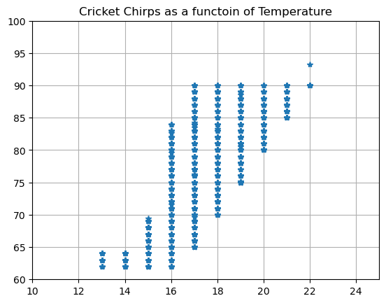
There seems to be an increase in the number of chirps as the temperature increases. We can put a straight line through this data using a polynomial fit
# Fit a linear trendline (polynomial of degree 1 = straight line)
coefficients = np.polyfit(x, y, 1)
coefficients
array([ 3.36808636, 17.96720331])The numbers we see here are the coefficients for the equation of the line. The line that fits our data is
\[ T = 3.36808636 C + 17.96720331 \]
Let’s see how we can plot this function in matplotlib.
# Define your x and y values

# Get your range of x values
x = np.arange(10,25,.5)
# Create your y values using your function
y = 3.36808636*x + 17.96720331

# The plot stuff pretty much looks the same!
plt.plot(x,y,'-')
plt.grid()
plt.xlim([10,25])
plt.ylim([60,100])
plt.title('Cricket Chirps as a function of Temperature')

plt.show()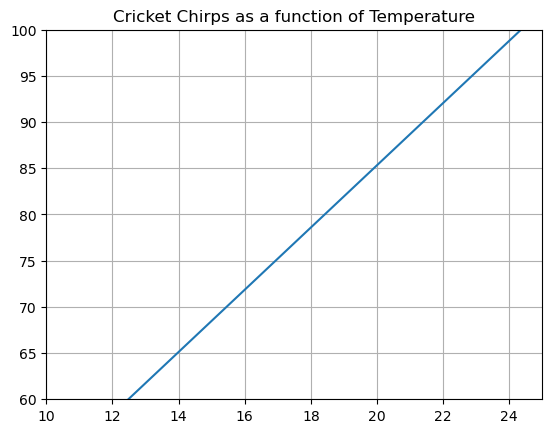
# Plot them together

yreal=np.array(DF['Temperature'])
xreal=np.array(DF['Chirps per Minute'])
x = np.arange(10,25,.5)
y = 3.36808636*x + 17.96720331


plt.plot(x,y,'-')
plt.plot(xreal,yreal,'*')
plt.grid()
plt.xlim([10,25])
plt.ylim([60,100])
plt.title('Cricket Chirps as a functoin of Temperature')

plt.show()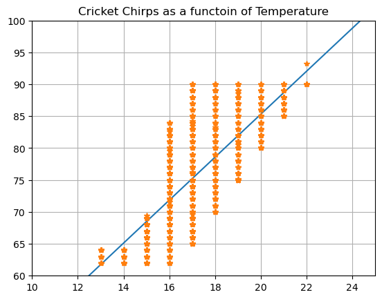
But now I can ask all sorts of questions!!!
- If I hear 20 chirps per minute what is a good estimate for the temperature?
- If the temperature is 70 degrees how many chirps should I expect to hear?
- For what range of numbers does my equation make sense?
# 1. If I hear 20 chirps per minute then x = 20
x = sp.symbols('x')
y = 3.36808636*x + 17.96720331
y.subs(x,20)
\(\displaystyle 85.32893051\)
1.
If there are 20 chirps per minute then it is about 85 degrees outside.
# 2. If the temperature is 70 degrees then y=70
# We need to find the inverse start with the expression - everything on the left hand side
x,y = sp.symbols('x,y')
my_expr = y - 3.36808636*x - 17.96720331

# Solve for the other variables so we get x=....
sp.solve(my_expr,x)
[0.296904500987914*y - 5.33454353290395]# Enter the new equation:
y = sp.symbols('y')
x = 0.296904500987914*y - 5.33454353290395
x.subs(y,70)\(\displaystyle 15.44877153625\)
2.
If it is 70 degrees outside then I should expect about 15 chirps per minute.
3.
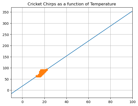
I know that my temperature can’t go infinitely high. Technically I could extend my linear fit way beyond where it is reasonable. This is why it is important to know what kind of numbers you might expect. Think about the following plot, what are the limitations on where we could use our prediction?
# Plot them together
xmin=-10
xmax= 100

yreal=np.array(DF['Temperature'])
xreal=np.array(DF['Chirps per Minute'])
x = np.arange(xmin,xmax,.5)
y = 3.36808636*x + 17.96720331


plt.plot(x,y,'-')
plt.plot(xreal,yreal,'*')
plt.grid()
plt.xlim([xmin,xmax])
plt.title('Cricket Chirps as a function of Temperature')

plt.show()